Usage
PhyKIT provides 100+ functions for processing and analyzing multiple sequence alignments and phylogenies. Functions span alignment quality assessment, tree manipulation, phylogenetic comparative methods, trait evolution modeling, introgression detection, and more.
Some help messages indicate that summary statistics are reported (e.g., bipartition_support_stats). Summary statistics include mean, median, 25th percentile, 75th percentile, minimum, maximum, standard deviation, and variance. These functions typically have a verbose option that allows users to get the underlying data used to calculate summary statistics.
Quick start
Here is a typical workflow showing a few common PhyKIT operations:
# Check alignment quality
phykit pis alignment.fa                  # count parsimony informative sites
phykit aot alignment.fa --json           # flag outlier taxa

# Summarize tree properties
phykit treeness species.tre              # treeness (internal/total branch length)
phykit dvmc species.tre                  # degree of violation of a molecular clock

# Phylogenetic comparative methods
phykit pgls -t species.tre -d traits.tsv \
    --response brain_size --predictor body_mass   # PGLS regression
phykit panova -t species.tre \
    --traits traits.tsv --pairwise                # phylogenetic ANOVA

# Visualize gene tree concordance
phykit qpie -t species.tre -g gene_trees.nwk \
    -o concordance.png --branch-labels            # quartet pie chart
General usage
Calling functions
phykit <command> [optional command arguments]
Command specific help messages can be viewed by adding a -h/--help argument after the command. For example, to see the help message for the command 'treeness', execute:
phykit treeness -h
# or
phykit treeness --help
Function aliases
Each function comes with aliases to save the user some key strokes. For example, to get the help message for the 'treeness' function, you can type:
phykit tness -h
Command line interfaces
As of version 1.2.0, all functions (including aliases) can be executed using a command line interface that starts with pk_. For example, instead of typing the previous command to get the help message of the treeness function, you can type:
pk_treeness -h
# or
pk_tness -h
All possible function names are specified at the top of each function section.
Functions by analytical category
The functions above are organized by input type. Below, the same functions are grouped by analytical purpose to help you find the right tool for your analysis.
Alignment quality & statistics
Alignment entropy: Shannon entropy across alignment sites
Alignment length: Length of an input alignment
Alignment length no gaps: Alignment length excluding gapped sites
Alignment outlier taxa: Identify outlier taxa in alignments
Column score: Column score for alignment quality
Composition per taxon: Nucleotide or amino acid composition per taxon
Compositional bias per site: Detect compositional bias across sites
Evolutionary rate per site: Site-specific evolutionary rate estimation
Guanine-cytosine (GC) content: GC content of an alignment
Identity matrix: Pairwise sequence identity heatmap
Occupancy per taxon: Taxon occupancy in alignment columns
Pairwise identity: Pairwise sequence identity in an alignment
Parsimony informative sites: Count parsimony informative sites
Plot alignment QC: Visual quality control plots for alignments
Relative composition variability: Composition variability across taxa
Relative composition variability, taxon: Per-taxon relative composition variability
Sum-of-pairs score: Sum-of-pairs alignment quality score
Variable sites: Count variable sites in an alignment
Alignment & dataset utilities
Alignment recoding: Recode alignment into reduced alphabets
Alignment subsampling: Randomly subsample genes, partitions, or sites
Create concatenation matrix: Concatenate multiple alignments into a supermatrix
Faidx: Extract entries from FASTA files
Mask alignment: Mask sites in an alignment
Occupancy filter: Filter alignments or trees by cross-file taxon occupancy (works with both FASTA and Newick)
Protein-to-nucleotide alignment: Thread nucleotide onto protein alignment
Rename FASTA entries: Rename entries in a FASTA file
Taxon groups: Group alignment or tree files by shared taxon sets (works with both FASTA and Newick)
Tree summary statistics
Bipartition support statistics: Summary statistics of bipartition support values
Degree of violation of the molecular clock: Measure molecular clock violation
Evolutionary rate: Calculate tree-based evolutionary rate
Faith's phylogenetic diversity: Sum of branch lengths spanning a community of tips
Internal branch statistics: Summary statistics of internal branch lengths
Lineage-through-time plot and gamma statistic: Lineage-through-time analysis and gamma statistic
Long branch score: Identify long branches in a tree
Patristic distances: Pairwise patristic distances between taxa
Terminal branch statistics: Summary statistics of terminal branch lengths
Tip-to-tip distance: Distance between two tips in a tree
Tip-to-tip node distance: Node distance between two tips
Total tree length: Sum of all branch lengths
Treeness: Ratio of internal to total branch lengths
Tree manipulation & utilities
Branch length multiplier: Multiply branch lengths by a factor
Chronogram: Time-calibrated tree with geological timescale (rectangular or circular)
Collapse bipartitions: Collapse low-support bipartitions
Internode labeler: Label internal nodes of a tree
Last common ancestor subtree: Extract subtree from LCA of specified taxa
Monophyly check: Test monophyly of a group of taxa
Nearest neighbor interchange: Generate NNI tree rearrangements
Print tree: Print ASCII representation of a tree
Prune tree: Prune taxa from a tree
Rename tree tips: Rename tip labels in a tree
Root tree: Root or reroot a tree
Subtree pruning and regrafting: Generate all SPR rearrangements for a specified subtree
Tip labels: Print tip labels of a tree
Transfer annotations: Transfer node annotations between trees (e.g., wASTRAL to RAxML/IQ-TREE)
Tree comparison & consensus
Consensus network: Consensus network from multiple trees
Consensus tree: Consensus tree from multiple trees
Cophylogenetic plot (tanglegram): Tanglegram for comparing two trees
Evolutionary tempo mapping: Detect rate-topology associations in gene trees
Kuhner-Felsenstein distance: Branch score distance between trees (topology + branch lengths)
NeighborNet: NeighborNet phylogenetic network from distance matrix (Bryant & Moulton 2004)
Polytomy testing: Test for polytomies in a tree
Quartet network: Quartet-based network visualization
Quartet pie chart: Phylogram with quartet concordance pie charts at internal nodes
Robinson-Foulds distance: Topological distance between trees
Spectral discordance decomposition: PCA ordination and clustering of gene tree topologies
Tree space: Visualize gene tree topology space via MDS, t-SNE, UMAP, or clustered distance heatmap
Introgression & gene flow
D-statistic (ABBA-BABA): Patterson's D-statistic for detecting introgression
DFOIL test: DFOIL test for detecting and polarizing introgression in a 5-taxon symmetric phylogeny
Discordance asymmetry: Test for asymmetric discordance (gene flow detection)
Hybridization analysis: Estimate reticulation events and localize hybridization on a species tree
Phylogenetic signal
Network signal: Phylogenetic signal on networks
Phylogenetic signal: Test for phylogenetic signal in traits (supports discordance-aware VCV with
-g)Trait correlation: Phylogenetic correlations between all pairs of traits with heatmap visualization
Trait evolution
Ancestral state reconstruction: Reconstruct ancestral character states
Character map: Map synapomorphies and homoplasies onto a phylogeny
Concordance-aware ASR: ASR incorporating gene tree discordance
Continuous trait evolution model comparison (fitContinuous): Compare continuous trait evolution models (supports discordance-aware VCV with
-g)Continuous trait mapping (contMap): Map continuous traits onto a phylogeny
Density map: Posterior density of stochastic character maps
Discrete trait evolution model comparison (fitDiscrete): Compare ER, SYM, ARD Mk models
Disparity through time (DTT): Disparity-through-time analysis with MDI statistic (Harmon et al. 2003)
Independent contrasts (PIC): Felsenstein's phylogenetically independent contrasts
Multi-regime OU models (OUwie): Multi-regime Ornstein-Uhlenbeck models
OU shift detection (l1ou): Detect OU regime shifts on a phylogeny
Parsimony score: Fitch parsimony score of a tree given an alignment
Phenogram (traitgram): Phenogram visualizing trait evolution
Phylogenetic heatmap: Phylogeny alongside a heatmap of numeric trait values
Phylogenetic imputation: Impute missing trait values using phylogenetic relationships
Rate heterogeneity test (multi-rate Brownian motion): Test for rate heterogeneity in trait evolution
SIMMAP summary: Per-branch SIMMAP summary with node posteriors (describe.simmap)
Stochastic character mapping (SIMMAP): Stochastic character mapping on a phylogeny
Threshold model: Felsenstein threshold model for trait correlation
Trait rate map: Per-branch evolutionary rate map for a continuous trait
Phylogenetic comparative methods
Phylo GWAS: Phylogenetic genome-wide association study
Phylogenetic ANOVA / MANOVA: Phylogenetic ANOVA or MANOVA using RRPP (Adams & Collyer 2018)
Phylogenetic GLM: Phylogenetic generalized linear model (supports discordance-aware VCV with
-g)Phylogenetic logistic regression: Phylogenetic logistic regression for binary traits (Ives & Garland 2010)
Phylogenetic ordination: Ordination incorporating phylogenetic structure (supports discordance-aware VCV with
-g)Phylogenetic path analysis: Compare causal DAGs via d-separation + PGLS (von Hardenberg & Gonzalez-Voyer 2013)
Phylogenetic regression (PGLS): Phylogenetic generalized least squares regression (supports discordance-aware VCV with
-g)Phylomorphospace: Phylomorphospace visualization
Evolutionary rate analysis
Covarying evolutionary rates: Detect covariation in evolutionary rates
Relative rate test: Relative rate test between lineages
Homology assessment
Hidden paralogy check: Check for hidden paralogy in gene trees
Spurious homolog identification: Identify spurious sequences in alignments
Saturation & model adequacy
Saturation: Test for substitution saturation
Treeness over RCV: Treeness over relative composition variability
Alignment-based functions
Alignment entropy
Function names: alignment_entropy; aln_entropy; entropy
Command line interface: pk_alignment_entropy; pk_aln_entropy; pk_entropy
Calculate alignment entropy.
Site-wise entropy is calculated using Shannon entropy. By default, PhyKIT reports the mean entropy across all sites in the alignment. With the -v/--verbose option, PhyKIT reports entropy for each site.
phykit alignment_entropy <alignment> [-v/--verbose] [--plot] [--plot-output <path>]
        [--fig-width <float>] [--fig-height <float>] [--dpi <int>] [--no-title] [--title <str>]
        [--legend-position <str>] [--ylabel-fontsize <float>] [--xlabel-fontsize <float>]
        [--title-fontsize <float>] [--axis-fontsize <float>] [--colors <str>] [--ladderize] [--cladogram] [--circular] [--color-file <file>] [--json]
Example output (default):
0.657
Example output (-v):
1       0.0
2       1.0
3       0.971
Options:
<alignment>: first argument after function name should be an alignment file
-v/--verbose: optional argument to print entropy for each site
--plot: save a per-site alignment entropy plot
--plot-output: output path for plot (default: alignment_entropy_plot.png)
--fig-width: figure width in inches (auto-scaled if omitted)
--fig-height: figure height in inches (auto-scaled if omitted)
--dpi: resolution in DPI (default: 300)
--no-title: hide the plot title
--title: custom title text
--legend-position: legend location (e.g., "upper right", "none" to hide)
--ylabel-fontsize: font size for y-axis labels; 0 to hide
--xlabel-fontsize: font size for x-axis labels; 0 to hide
--title-fontsize: font size for the title
--axis-fontsize: font size for axis labels
--colors: comma-separated colors (hex or named)
--ladderize: ladderize (sort) the tree before plotting
--cladogram: draw cladogram (equal branch lengths, tips aligned) instead of phylogram
--circular: draw circular (radial/fan) phylogram instead of rectangular
--color-file: color annotation file for tip labels, clade ranges, and branch colors (iTOL-inspired TSV format)
--json: optional argument to print results as JSON
Alignment length

Function names: alignment_length; aln_len; al
Command line interface: pk_alignment_length; pk_aln_len; pk_al
Length of an input alignment is calculated using this function.
Longer alignments are associated with a strong phylogenetic signal.
The association between alignment length and phylogenetic signal was determined by Shen et al., Genome Biology and Evolution (2016), doi: 10.1093/gbe/evw179.
phykit aln_len <alignment> [--json]
Options:
<alignment>: first argument after function name should be an alignment file
--json: optional argument to print results as JSON
Alignment length no gaps
Function names: alignment_length_no_gaps; aln_len_no_gaps; alng
Command line interface: pk_alignment_length_no_gaps; pk_aln_len_no_gaps; pk_alng
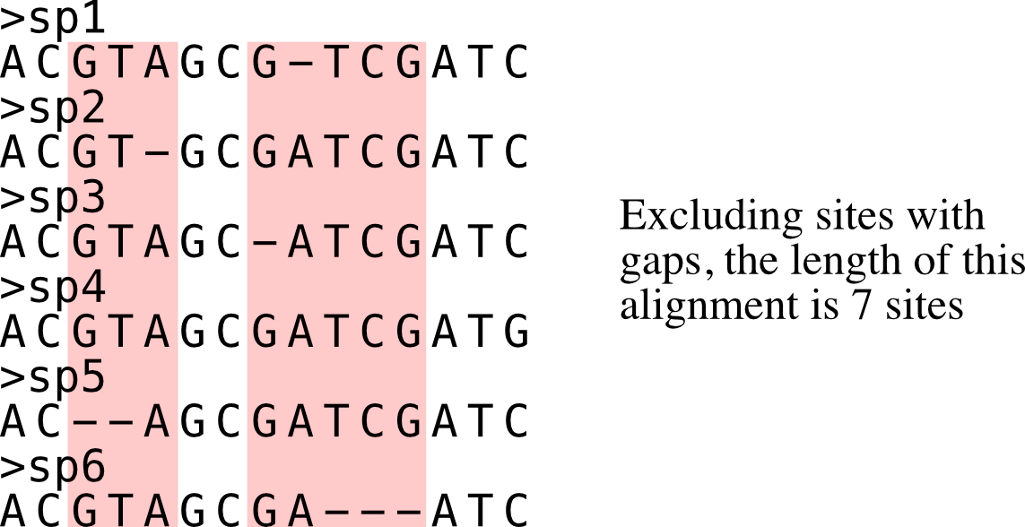
Calculate alignment length excluding sites with gaps.
Longer alignments when excluding sites with gaps are associated with a strong phylogenetic signal.
PhyKIT reports three tab delimited values: col1: number of sites without gaps col2: total number of sites col3: percentage of sites without gaps
The association between alignment length when excluding sites with gaps and phylogenetic signal was determined by Shen et al., Genome Biology and Evolution (2016), doi: 10.1093/gbe/evw179.
phykit aln_len_no_gaps <alignment> [--json]
Options:
<alignment>: first argument after function name should be an alignment file
--json: optional argument to print results as JSON
Alignment outlier taxa
Function names: alignment_outlier_taxa; outlier_taxa; aot
Command line interface: pk_alignment_outlier_taxa; pk_outlier_taxa; pk_aot
Identify potential outlier taxa in an alignment and explicitly report why each taxon was flagged.
The following features are evaluated per taxon:
1) gap_rate: fraction of gap/ambiguous symbols
2) occupancy: fraction of valid symbols
3) composition_distance: Euclidean distance from the median composition profile
4) long_branch_proxy: mean pairwise sequence distance to other taxa
5) rcvt: relative composition variability per taxon
6) entropy_burden: average site entropy over this taxon's valid positions
If a taxon exceeds one or more feature-specific thresholds, PhyKIT reports the exact feature(s), observed value(s), threshold(s), and explanation(s) for the flag.
phykit alignment_outlier_taxa <alignment> [--gap-z <float>] [--composition-z <float>] [--distance-z <float>] [--rcvt-z <float>] [--occupancy-z <float>] [--entropy-z <float>] [--json]
Example output:
features_evaluated      gap_rate,occupancy,composition_distance,long_branch_proxy,rcvt,entropy_burden
thresholds      gap_rate>0.0;occupancy<0.4;composition_distance>0.1;long_branch_proxy>0.4181;rcvt>0.0095;entropy_burden>0.35
taxon_d composition_distance=1.3454>0.1;long_branch_proxy=1.0>0.4181    Unusual sequence composition profile relative to other taxa. | High mean pairwise sequence distance to other taxa.
taxon_e gap_rate=0.6>0.0;occupancy=0.4<0.4      High fraction of gap/ambiguous symbols compared to other taxa. | Low fraction of valid symbols compared to other taxa.
Options:
<alignment>: first argument after function name should be an alignment file
--gap-z: z-threshold used for high-gap outlier detection (default: 3.0)
--composition-z: z-threshold used for composition-distance outlier detection (default: 3.0)
--distance-z: z-threshold used for long-branch-proxy outlier detection (default: 3.0)
--rcvt-z: z-threshold used for RCVT outlier detection (default: 3.0)
--occupancy-z: z-threshold used for low-occupancy outlier detection (default: 3.0)
--entropy-z: z-threshold used for entropy-burden outlier detection (default: 3.0)
--json: optional argument to print results as JSON
Alignment recoding
Function names: alignment_recoding; aln_recoding; recode
Command line interface: pk_alignment_recoding; pk_aln_recoding; pk_recode
Recode alignments using reduced character states.
Alignments can be recoded using established or custom recoding schemes. Recoding schemes are specified using the -c/--code argument. Custom recoding schemes can be used and should be formatted as a two column file wherein the first column is the recoded character and the second column is the character in the alignment.
phykit alignment_recoding <fasta> [-c/--code <code>] [--json]
Codes for which recoding scheme to use:
RY-nucleotide
R = purines (i.e., A and G)
Y = pyrimidines (i.e., T and C)
SandR-6
0 = A, P, S, and T
1 = D, E, N, and G
2 = Q, K, and R
3 = M, I, V, and L
4 = W and C
5 = F, Y, and H
KGB-6
0 = A, G, P, and S
1 = D, E, N, Q, H, K, R, and T
2 = M, I, and L
3 = W
4 = F and Y
5 = C and V
Dayhoff-6
0 = A, G, P, S, and T
1 = D, E, N, and Q
2 = H, K, and R
3 = I, L, M, and V
4 = F, W, and Y
5 = C
Dayhoff-9
0 = D, E, H, N, and Q
1 = I, L, M, and V
2 = F and Y
3 = A, S, and T
4 = K and R
5 = G
6 = P
7 = C
8 = W
Dayhoff-12
0 = D, E, and Q
1 = M, L, I, and V
2 = F and Y
3 = K, H, and R
4 = G
5 = A
6 = P
7 = S
8 = T
9 = N
A = W
B = C
Dayhoff-15
0 = D, E, and Q
1 = M and L
2 = I and V
3 = F and Y
4 = G
5 = A
6 = P
7 = S
8 = T
9 = N
A = K
B = H
C = R
D = W
E = C
Dayhoff-18
0 = F and Y
1 = M and L
2 = I
3 = V
4 = G
5 = A
6 = P
7 = S
8 = T
9 = D
A = E
B = Q
C = N
D = K
E = H
F = R
G = W
H = C
Options:
<alignment>: first argument after function name should be an alignment file
-c/--code: argument to specify the recoding scheme to use
--json: optional argument to print results as JSON
Alignment subsampling
Function names: alignment_subsample; aln_subsample; subsample
Command line interface: pk_alignment_subsample; pk_aln_subsample; pk_subsample
Randomly subsample genes, partitions, or sites from phylogenomic datasets. Supports three modes:
genes: Given a file listing alignment paths, randomly select N of them.
partitions: Given a supermatrix + RAxML-style partition file, randomly select N partitions and extract their columns into a new alignment.
sites: Given a single alignment, randomly select N columns.
Sampling can be without replacement (default, for jackknife-style tests) or
with replacement using --bootstrap (for gene/site bootstrapping).
Use --seed for reproducibility.
# Subsample 50 genes from a list of 200
phykit alignment_subsample --mode genes -l gene_list.txt --number 50 -o sub50

# Subsample 50% of partitions from a supermatrix
phykit alignment_subsample --mode partitions -a concat.fa -p concat.partition \
    --fraction 0.5 --seed 42 -o sub50pct

# Bootstrap-resample sites from an alignment
phykit alignment_subsample --mode sites -a alignment.fa \
    --number 500 --bootstrap --seed 1 -o boot1
Options:
--mode: subsampling mode: genes, partitions, or sites (required)
-a/--alignment: input alignment file in FASTA format (required for partitions and sites modes)
-l/--list: file listing alignment paths, one per line (required for genes mode)
-p/--partition: RAxML-style partition file (required for partitions mode)
--number: exact number of items to select (mutually exclusive with --fraction)
--fraction: fraction of items to select, 0.0 to 1.0 (mutually exclusive with --number)
--bootstrap: sample with replacement (default: without replacement)
--seed: random seed for reproducibility
-o/--output: output file prefix (default: subsampled)
--json: optional argument to print results as JSON
Column score
Function names: column_score; cs
Command line interface: pk_column_score; pk_cs
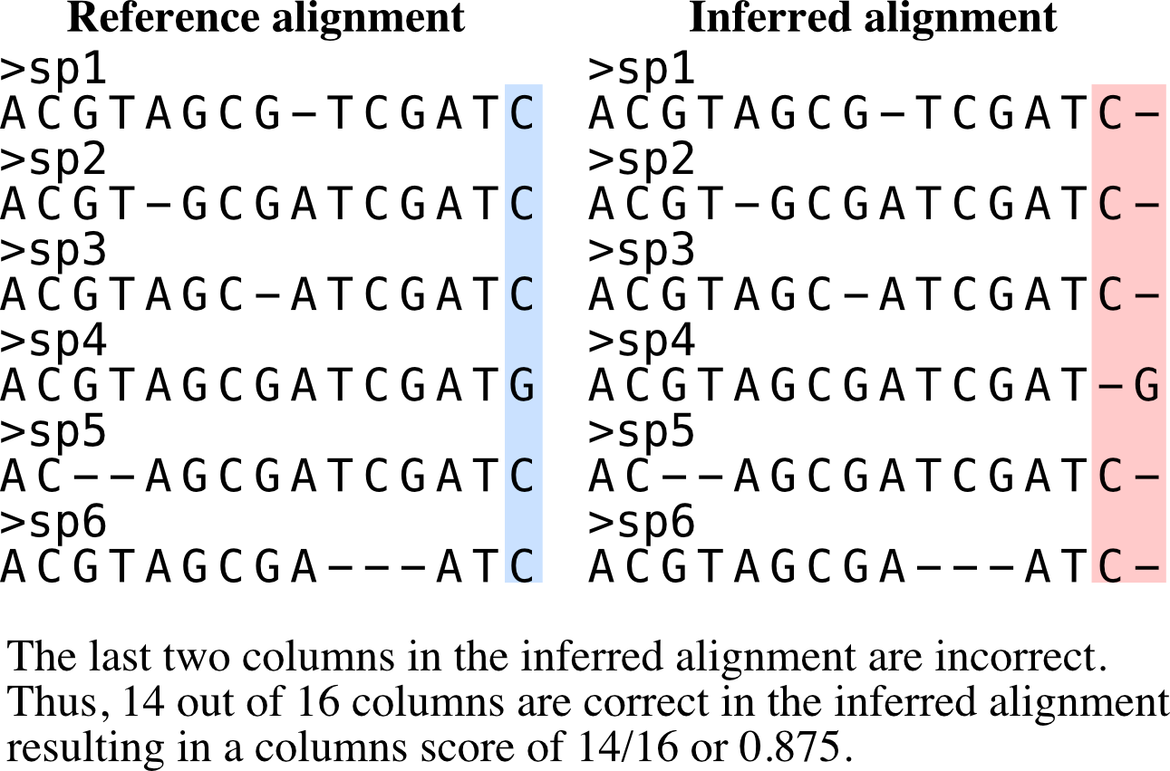
Calculates column score.
Column score is an accuracy metric for a multiple alignment relative to a reference alignment. It is calculated by summing the correctly aligned columns over all columns in an alignment. Thus, values range from 0 to 1 and higher values indicate more accurate alignments.
Column score is calculated following Thompson et al., Nucleic Acids Research (1999), doi: 10.1093/nar/27.13.2682.
phykit column_score <alignment> --reference <reference_alignment> [--json]
Options:
<alignment>: first argument after function name should be a query
fasta alignment file to be scored for accuracy
-r/--reference: reference alignment to compare the query alignment
to
--json: optional argument to print results as JSON
Composition per taxon
Function names: composition_per_taxon; comp_taxon; comp_tax
Command line interface: pk_composition_per_taxon; pk_comp_taxon; pk_comp_tax
Calculate sequence composition per taxon in an alignment.
Composition is reported as semicolon-separated symbol:frequency pairs for each taxon. Frequencies are calculated from valid (non-gap/non-ambiguous) characters. Symbol order is alphabetical.
phykit composition_per_taxon <alignment> [--json]
Example output:
1       A:0.4;C:0.0;G:0.2;T:0.4
2       A:0.5;C:0.0;G:0.25;T:0.25
Options:
<alignment>: first argument after function name should be an alignment file
--json: optional argument to print results as JSON
Compositional bias per site
Function names: compositional_bias_per_site; comp_bias_per_site; cbps
Command line interface: pk_compositional_bias_per_site; pk_comp_bias_per_site; pk_cbps
Calculates compositional bias per site in an alignment.
Site-wise chi-squared tests are conducted in an alignment to
detect compositional biases. PhyKIT outputs four columns:
col 1: index in alignment
col 2: chi-squared statistic (higher values indicate greater bias)
col 3: multi-test corrected p-value (Benjamini-Hochberg false discovery rate procedure)
col 4: uncorrected p-value
phykit comp_bias_per_site <alignment> [--plot] [--plot-output <path>]
        [--fig-width <float>] [--fig-height <float>] [--dpi <int>] [--no-title] [--title <str>]
        [--legend-position <str>] [--ylabel-fontsize <float>] [--xlabel-fontsize <float>]
        [--title-fontsize <float>] [--axis-fontsize <float>] [--colors <str>] [--ladderize] [--cladogram] [--circular] [--color-file <file>] [--json]
Options:
<alignment>: first argument after function name should be a query
fasta alignment to calculate the site-wise compositional bias of
--plot: save a Manhattan-style plot of site-wise compositional bias
--plot-output: output path for plot (default: compositional_bias_per_site_plot.png)
--fig-width: figure width in inches (auto-scaled if omitted)
--fig-height: figure height in inches (auto-scaled if omitted)
--dpi: resolution in DPI (default: 300)
--no-title: hide the plot title
--title: custom title text
--legend-position: legend location (e.g., "upper right", "none" to hide)
--ylabel-fontsize: font size for y-axis labels; 0 to hide
--xlabel-fontsize: font size for x-axis labels; 0 to hide
--title-fontsize: font size for the title
--axis-fontsize: font size for axis labels
--colors: comma-separated colors (hex or named)
--ladderize: ladderize (sort) the tree before plotting
--cladogram: draw cladogram (equal branch lengths, tips aligned) instead of phylogram
--circular: draw circular (radial/fan) phylogram instead of rectangular
--color-file: color annotation file for tip labels, clade ranges, and branch colors (iTOL-inspired TSV format)
--json: optional argument to print results as JSON
Create concatenation matrix
Function names: create_concatenation_matrix; create_concat; cc
Command line interface: pk_create_concatenation_matrix; pk_create_concat; pk_cc
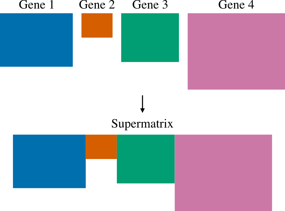
Create a concatenated alignment file. This function is used to help in the construction of multi-locus data matrices.
PhyKIT will output three files: 1) A fasta file with '.fa' appended to the prefix specified with the -p/--prefix parameter. 2) A partition file ready for input into RAxML or IQ-tree. 3) An occupancy file that summarizes the taxon occupancy per sequence.
phykit create_concat -a <file> -p <string> [--threshold <float>] [--plot-occupancy] [--plot-output <path>]
        [--fig-width <float>] [--fig-height <float>] [--dpi <int>] [--no-title] [--title <str>]
        [--legend-position <str>] [--ylabel-fontsize <float>] [--xlabel-fontsize <float>]
        [--title-fontsize <float>] [--axis-fontsize <float>] [--colors <str>] [--ladderize] [--cladogram] [--circular] [--color-file <file>] [--json]
Options:
-a/--alignment: alignment list file. File should contain a single column list of alignment
sequence files to concatenate into a single matrix. Provide path to files relative to
working directory or provide absolute path.
-p/--prefix: prefix of output files
--threshold: minimum fraction of informative (non-gap, non-ambiguous) sites across the
concatenated alignment for a taxon to be included. Taxa whose effective occupancy falls
below this value are excluded from the output. Set to 0 to disable filtering
(default: 0).
--plot-occupancy: optional argument to output an occupancy map figure where
x-axis shows concatenated positions with gene boundaries and y-axis shows taxa
sorted by total occupancy. Colors denote represented characters, gap/ambiguous
characters in present genes, and fully absent gene blocks.
--plot-output: optional custom output path for occupancy map figure
(default: <prefix>.occupancy.png).
--fig-width: figure width in inches (auto-scaled if omitted)
--fig-height: figure height in inches (auto-scaled if omitted)
--dpi: resolution in DPI (default: 300)
--no-title: hide the plot title
--title: custom title text
--legend-position: legend location (e.g., "upper right", "none" to hide)
--ylabel-fontsize: font size for y-axis labels; 0 to hide
--xlabel-fontsize: font size for x-axis labels; 0 to hide
--title-fontsize: font size for the title
--axis-fontsize: font size for axis labels
--colors: comma-separated colors (hex or named)
--ladderize: ladderize (sort) the tree before plotting
--cladogram: draw cladogram (equal branch lengths, tips aligned) instead of phylogram
--circular: draw circular (radial/fan) phylogram instead of rectangular
--color-file: color annotation file for tip labels, clade ranges, and branch colors (iTOL-inspired TSV format)
--json: optional argument to print summary metadata as JSON
Evolutionary Rate per Site
Function names: evolutionary_rate_per_site; evo_rate_per_site; erps
Command line interface: pk_evolutionary_rate_per_site; pk_evo_rate_per_site; pk_erps
Estimate evolutionary rate per site.
Evolutionary rate per site is one minus the sum of squared frequency of different characters at a given site. Values may range from 0 (slow evolving; no diversity at the given site) to 1 (fast evolving; all characters appear only once).
phykit evo_rate_per_site <alignment> [--plot] [--plot-output <path>]
        [--fig-width <float>] [--fig-height <float>] [--dpi <int>] [--no-title] [--title <str>]
        [--legend-position <str>] [--ylabel-fontsize <float>] [--xlabel-fontsize <float>]
        [--title-fontsize <float>] [--axis-fontsize <float>] [--colors <str>] [--ladderize] [--cladogram] [--circular] [--color-file <file>] [--json]
Options:
<alignment>: first argument after function name should be a query
fasta alignment to calculate the site-wise evolutionary rate of
--plot: save a per-site evolutionary-rate plot
--plot-output: output path for plot (default: evolutionary_rate_per_site_plot.png)
--fig-width: figure width in inches (auto-scaled if omitted)
--fig-height: figure height in inches (auto-scaled if omitted)
--dpi: resolution in DPI (default: 300)
--no-title: hide the plot title
--title: custom title text
--legend-position: legend location (e.g., "upper right", "none" to hide)
--ylabel-fontsize: font size for y-axis labels; 0 to hide
--xlabel-fontsize: font size for x-axis labels; 0 to hide
--title-fontsize: font size for the title
--axis-fontsize: font size for axis labels
--colors: comma-separated colors (hex or named)
--ladderize: ladderize (sort) the tree before plotting
--cladogram: draw cladogram (equal branch lengths, tips aligned) instead of phylogram
--circular: draw circular (radial/fan) phylogram instead of rectangular
--color-file: color annotation file for tip labels, clade ranges, and branch colors (iTOL-inspired TSV format)
--json: optional argument to print results as JSON
Faidx

Function names: faidx; get_entry; ge
Command line interface: pk_faidx; pk_get_entry; pk_ge
Extracts a sequence entry from a fasta file.
This function works similarly to the faidx function in samtools, but does not require an indexing step.
To obtain multiple entries, input multiple entries separated by a comma (,). For example, if you want entries named "seq_0" and "seq_1", the string "seq_0,seq_1" should be associated with the -e argument.
phykit faidx <fasta> -e/--entry <fasta entry> [--json]
Options:
<fasta>: first argument after function name should be a fasta file
-e/--entry: entry name to be extracted from the inputted fasta file
--json: optional argument to print results as JSON
Guanine-cytosine (GC) content

Function names: gc_content; gc
Command line interface: pk_gc_content; pk_gc
Calculate GC content of a fasta file.
GC content is negatively correlated with phylogenetic signal.
If there are multiple entries, use the -v/--verbose option to determine the GC content of each fasta entry separately. The association between GC content and phylogenetic signal was determined by Shen et al., Genome Biology and Evolution (2016), doi: 10.1093/gbe/evw179.
phykit gc_content <fasta> [-v/--verbose] [--json]
Options:
<fasta>: first argument after function name should be a fasta file
-v/--verbose: optional argument to print the GC content of each fasta
entry
--json: optional argument to print results as JSON
Identity matrix
Function names: identity_matrix; id_matrix; seqid
Command line interface: pk_identity_matrix; pk_id_matrix; pk_seqid
Compute a pairwise sequence identity matrix from an alignment and plot it as a clustered heatmap.
For each pair of taxa, identity is defined as the fraction of non-gap, non-ambiguous columns that are identical. Gaps, '?', 'N', 'X', and '*' in either sequence cause a column to be skipped.
The matrix can be displayed as identity (default) or p-distance (1 - identity) using --metric. Ordering can be by hierarchical clustering (default), tree tip order (--sort tree --tree <file>), or alphabetical (--sort alpha).
phykit identity_matrix -a <alignment> -o <output>
        [--metric identity|p-distance] [--tree <file>]
        [--sort alpha|cluster|tree] [--partition <file>] [--json]
        [--fig-width <float>] [--fig-height <float>] [--dpi <int>]
        [--no-title] [--title <str>]
        [--ylabel-fontsize <float>] [--xlabel-fontsize <float>]
        [--title-fontsize <float>] [--axis-fontsize <float>]
Options:
-a/--alignment: alignment file (FASTA or other supported format)
-o/--output: output figure path (.png, .pdf, .svg)
--metric: 'identity' (fraction matching) or 'p-distance' (1 - identity); default: identity
--tree: tree file for tree-guided ordering (Newick format)
--sort: ordering method: 'cluster' (hierarchical), 'tree' (requires --tree), or 'alpha' (alphabetical); default: cluster
--partition: RAxML-style partition file (reserved for future use)
--json: output structured JSON instead of plain text
--fig-width: figure width in inches (auto-scaled if omitted)
--fig-height: figure height in inches (auto-scaled if omitted)
--dpi: resolution in DPI (default: 300)
--no-title: hide the plot title
--title: custom title text
--ylabel-fontsize: font size for y-axis labels; 0 to hide
--xlabel-fontsize: font size for x-axis labels; 0 to hide
--title-fontsize: font size for the title
--axis-fontsize: font size for axis labels
Mask alignment
Function names: mask_alignment; mask_aln; mask
Command line interface: pk_mask_alignment; pk_mask_aln; pk_mask
Mask alignment sites based on threshold criteria.
Sites are retained when they pass all active thresholds: maximum gap fraction, minimum occupancy, and maximum site entropy.
phykit mask_alignment <alignment> [-g/--max_gap <float>] [-o/--min_occupancy <float>] [-e/--max_entropy <float>] [--json]
Options:
<alignment>: first argument after function name should be an alignment file
-g/--max_gap: maximum allowed fraction of missing/invalid characters at a site (default: 1.0)
-o/--min_occupancy: minimum required occupancy at a site (default: 0.0)
-e/--max_entropy: maximum allowed site entropy (default: no filter)
--json: optional argument to print results as JSON
Occupancy filter
Function names: occupancy_filter; occ_filter; filter_occupancy
Command line interface: pk_occupancy_filter; pk_occ_filter; pk_filter_occupancy
Filter alignments and/or trees by cross-file taxon occupancy. Given a list of alignment or tree files, counts how many files each taxon appears in and retains only taxa meeting a minimum threshold. Outputs filtered copies of each input file.
This is useful for phylogenomics workflows where you want to ensure all taxa in your dataset are present in at least N genes before concatenation or downstream analysis. For FASTA files, sequences of removed taxa are dropped. For tree files, tips of removed taxa are pruned.
Example: Given 10 alignment files and -t 0.5 (the default), only
taxa present in at least 5 of the 10 alignments will be retained. New
filtered alignment files are written with the removed taxa excluded.
Threshold interpretation:
Values between 0 and 1 (inclusive) are treated as a fraction of the total number of files. For example,
-t 0.5means 50% of files;-t 1.0means 100% (taxon must be in every file).Values greater than 1 are treated as an absolute count. For example,
-t 5means the taxon must appear in at least 5 files.The default is
0.5(50% occupancy).
# Keep taxa in at least 50% of files (default)
phykit occupancy_filter -l alignment_list.txt

# Keep taxa in all files (100% occupancy)
phykit occupancy_filter -l alignment_list.txt -t 1.0

# Keep taxa in at least 20 files
phykit occupancy_filter -l alignment_list.txt -t 20

# Filter trees instead of alignments
phykit occ_filter -l tree_list.txt -f trees -t 0.5 -o filtered_trees/
phykit occupancy_filter -l <file_list> [-f/--format fasta|trees]
    [-t/--threshold <float>] [-o/--output-dir <dir>] [--suffix <str>] [--json]
Options:
-l/--list: file listing paths to alignment or tree files, one per line (required)
-f/--format: input file format — fasta (default) or trees
-t/--threshold: minimum occupancy to retain a taxon. Values between 0 and 1 (inclusive) are treated as a fraction (e.g., 0.5 = 50%, 1.0 = 100%); values > 1 are treated as an absolute count (default: 0.5)
-o/--output-dir: directory for filtered output files (default: same directory as input)
--suffix: suffix added to output filenames before the extension (default: .filtered)
--json: output results as JSON
Occupancy per taxon
Function names: occupancy_per_taxon; occupancy_taxon; occ_tax
Command line interface: pk_occupancy_per_taxon; pk_occupancy_taxon; pk_occ_tax
Calculate occupancy per taxon in an alignment.
Occupancy is the fraction of valid (non-gap/non-ambiguous) characters for each taxon.
phykit occupancy_per_taxon <alignment> [--json]
Example output:
1       0.8333
2       0.6667
Options:
<alignment>: first argument after function name should be an alignment file
--json: optional argument to print results as JSON
Pairwise identity

Function names: pairwise_identity; pairwise_id; pi
Command line interface: pk_pairwise_identity; pk_pairwise_id; pk_pi
Calculate the average pairwise identity among sequences.
Pairwise identities can be used as proxies for the evolutionary rate of sequences.
Pairwise identity is defined as the number of identical columns (including gaps) between two aligned sequences divided by the number of columns in the alignment. Summary statistics are reported unless used with the verbose option in which all pairwise identities will be reported.
An example of pairwise identities being used as a proxy for evolutionary rate can be found here: Chen et al. Genome Biology and Evolution (2017), doi: 10.1093/gbe/evx147.
phykit pairwise_identity <alignment> [-v/--verbose] [-e/--exclude_gaps] [--plot] [--plot-output <file>]
        [--fig-width <float>] [--fig-height <float>] [--dpi <int>] [--no-title] [--title <str>]
        [--legend-position <str>] [--ylabel-fontsize <float>] [--xlabel-fontsize <float>]
        [--title-fontsize <float>] [--axis-fontsize <float>] [--colors <str>] [--ladderize] [--cladogram] [--circular] [--color-file <file>] [--json]
Options:
<alignment>: first argument after function name should be an alignment file
-v/--verbose: optional argument to print identity per pair
-e/--exclude_gaps: if a site has a gap, ignore it
--plot: save a clustered pairwise-identity heatmap
--plot-output: output path for heatmap (default: pairwise_identity_heatmap.png)
--fig-width: figure width in inches (auto-scaled if omitted)
--fig-height: figure height in inches (auto-scaled if omitted)
--dpi: resolution in DPI (default: 300)
--no-title: hide the plot title
--title: custom title text
--legend-position: legend location (e.g., "upper right", "none" to hide)
--ylabel-fontsize: font size for y-axis labels; 0 to hide
--xlabel-fontsize: font size for x-axis labels; 0 to hide
--title-fontsize: font size for the title
--axis-fontsize: font size for axis labels
--colors: comma-separated colors (hex or named)
--ladderize: ladderize (sort) the tree before plotting
--cladogram: draw cladogram (equal branch lengths, tips aligned) instead of phylogram
--circular: draw circular (radial/fan) phylogram instead of rectangular
--color-file: color annotation file for tip labels, clade ranges, and branch colors (iTOL-inspired TSV format)
--json: optional argument to print results as JSON
Parsimony informative sites
Function names: parsimony_informative_sites; pis
Command line interface: pk_parsimony_informative_sites; pk_pis
Calculate the number and percentage of parsimony informative sites in an alignment.
The number of parsimony informative sites in an alignment is associated with a strong phylogenetic signal.
PhyKIT reports three tab delimited values: col1: number of parsimony informative sites col2: total number of sites col3: percentage of parsimony informative sites
The association between the number of parsimony informative sites and phylogenetic signal was determined by Shen et al., Genome Biology and Evolution (2016), doi: 10.1093/gbe/evw179 and Steenwyk et al., PLOS Biology (2020), doi: 10.1371/journal.pbio.3001007.
phykit parsimony_informative_sites <alignment> [--json]
Options:
<alignment>: first argument after function name should be an alignment file
--json: optional argument to print results as JSON
Phylo GWAS
Function names: phylo_gwas; pgwas
Command line interface: pk_phylo_gwas; pk_pgwas
Phylogenetic genome-wide association study following the Pease et al. (2016) approach. Performs per-site association tests between alignment columns and a phenotype, applies Benjamini-Hochberg FDR correction, optionally classifies significant associations as monophyletic or polyphyletic using a phylogenetic tree, and produces a Manhattan plot.
Categorical phenotypes use Fisher's exact test (2 groups) or chi-squared test (>2 groups). Continuous phenotypes use point-biserial correlation. Only biallelic sites are tested; invariant and multiallelic sites are skipped. Sites with gaps or ambiguous characters are also skipped.
phykit phylo_gwas -a <alignment> -d <phenotype> -o <output>
  [-t <tree>] [-p <partition>] [--alpha 0.05]
  [--exclude-monophyletic] [--csv <file>] [--json]
Options:
-a/--alignment: FASTA alignment file
-d/--phenotype: two-column TSV file (taxon<tab>phenotype)
-o/--output: output Manhattan plot path
-t/--tree: optional Newick tree for monophyletic/polyphyletic classification
-p/--partition: optional RAxML-style partition file for gene annotations
--alpha: FDR significance threshold (default: 0.05)
--exclude-monophyletic: exclude monophyletic associations from results
--dot-size: scale factor for dot size in the Manhattan plot (default: 1.0; use 2.0 for double, 0.5 for half)
--csv: output per-site results as CSV to the specified file
--fig-width: figure width in inches (auto-scaled if omitted)
--fig-height: figure height in inches (auto-scaled if omitted)
--dpi: resolution in DPI (default: 300)
--no-title: hide the plot title
--title: custom title text
--legend-position: legend location (e.g., "upper right", "none")
--colors: comma-separated colors (hex or named)
--json: optional argument to print results as JSON
Plot alignment QC
Function names: plot_alignment_qc; plot_qc; paqc
Command line interface: pk_plot_alignment_qc; pk_plot_qc; pk_paqc
Generate a multi-panel alignment quality-control plot.
The figure includes:
1) occupancy per taxon
2) gap rate per taxon
3) composition distance vs long-branch proxy scatter
4) count of flagged outliers by feature
Outlier evaluation uses the same features as alignment_outlier_taxa:
gap_rate, occupancy, composition_distance, long_branch_proxy,
rcvt, and entropy_burden.
phykit plot_alignment_qc <alignment> [-o/--output <path>] [--width <float>] [--height <float>] [--dpi <int>] [--gap-z <float>] [--composition-z <float>] [--distance-z <float>] [--rcvt-z <float>] [--occupancy-z <float>] [--entropy-z <float>] [--json]
Options:
<alignment>: first argument after function name should be an alignment file
-o/--output: output image path (default: alignment_qc.png)
--width: figure width in inches (default: 14.0)
--height: figure height in inches (default: 10.0)
--dpi: output image DPI (default: 300)
--gap-z: z-threshold for gap-rate outliers (default: 3.0)
--composition-z: z-threshold for composition-distance outliers (default: 3.0)
--distance-z: z-threshold for long-branch-proxy outliers (default: 3.0)
--rcvt-z: z-threshold for RCVT outliers (default: 3.0)
--occupancy-z: z-threshold for low-occupancy outliers (default: 3.0)
--entropy-z: z-threshold for entropy-burden outliers (default: 3.0)
--json: optional argument to print plot metadata and outlier summary as JSON
Protein-to-nucleotide alignment
Function names: thread_dna; pal2nal; p2n
Command line interface: pk_thread_dna; pk_pal2nal; pk_p2n
Thread DNA sequence onto a protein alignment to create a codon-based alignment.
This function requires that input alignments be in fasta format. Codon alignments are then printed to stdout. Note, paired sequences are assumed to have the same name between the protein and nucleotide file. The order does not matter.
To thread nucleotide sequences over a trimmed amino acid alignment, provide PhyKIT with a log file specifying which sites have been trimmed and which have been kept. The log file must be formatted the same as the log files outputted by the alignment trimming toolkit ClipKIT (see -l in ClipKIT documentation.) Details about ClipKIT can be seen here: https://github.com/JLSteenwyk/ClipKIT.
If using a ClipKIT log file, the untrimmed protein alignment should be provided in the -p/--protein argument.
phykit thread_dna -p <file> -n <file> [-s] [--json]
Options:
-p/--protein: protein alignment file
-n/--nucleotide: nucleotide sequence file
-c/--clipkit_log: clipkit outputted log file
-s/--stop: if used, stop codons will be removed from the output
--json: optional argument to print results as JSON
Relative composition variability
Function names: relative_composition_variability; rel_comp_var; rcv
Command line interface: pk_relative_composition_variability; pk_rel_comp_var; pk_rcv
Calculate RCV (relative composition variability) for an alignment.
Lower RCV values are thought to be desirable because they represent a lower composition bias in an alignment. Statistically, RCV describes the average variability in sequence composition among taxa.
RCV is calculated following Phillips and Penny, Molecular Phylogenetics and Evolution (2003), doi: 10.1016/S1055-7903(03)00057-5.
RCV calculations are case-insensitive. Gap and ambiguous characters are excluded from composition counts and correction terms, and each taxon is normalized by its valid (non-excluded) sequence length.
phykit relative_composition_variability <alignment> [--json]
Options:
<alignment>: first argument after function name should be an alignment file
--json: optional argument to print results as JSON
Relative composition variability, taxon
Function names: relative_composition_variability_taxon; rel_comp_var_taxon; rcvt
Command line interface: pk_relative_composition_variability_taxon; pk_rel_comp_var_taxon; pk_rcvt
Calculate RCVT (relative composition variability, taxon) for an alignment.
RCVT is the relative composition variability metric for individual taxa. This facilitates identifying specific taxa that may have compositional biases. Lower RCVT values are more desirable because they indicate a lower composition bias for a given taxon in an alignment.
RCVT calculations are case-insensitive and exclude gap/ambiguous symbols from composition counts and normalization.
phykit relative_composition_variability_taxon <alignment> [--plot] [--plot-output <path>]
        [--fig-width <float>] [--fig-height <float>] [--dpi <int>] [--no-title] [--title <str>]
        [--legend-position <str>] [--ylabel-fontsize <float>] [--xlabel-fontsize <float>]
        [--title-fontsize <float>] [--axis-fontsize <float>] [--colors <str>] [--ladderize] [--cladogram] [--circular] [--color-file <file>] [--json]
Options:
<alignment>: first argument after function name should be an alignment file
--plot: optional argument to generate an RCVT per-taxon barplot
--plot-output: output path for the RCVT plot (default: rcvt_plot.png)
--fig-width: figure width in inches (auto-scaled if omitted)
--fig-height: figure height in inches (auto-scaled if omitted)
--dpi: resolution in DPI (default: 300)
--no-title: hide the plot title
--title: custom title text
--legend-position: legend location (e.g., "upper right", "none" to hide)
--ylabel-fontsize: font size for y-axis labels; 0 to hide
--xlabel-fontsize: font size for x-axis labels; 0 to hide
--title-fontsize: font size for the title
--axis-fontsize: font size for axis labels
--colors: comma-separated colors (hex or named)
--ladderize: ladderize (sort) the tree before plotting
--cladogram: draw cladogram (equal branch lengths, tips aligned) instead of phylogram
--circular: draw circular (radial/fan) phylogram instead of rectangular
--color-file: color annotation file for tip labels, clade ranges, and branch colors (iTOL-inspired TSV format)
--json: optional argument to print results as JSON
Rename FASTA entries
Function names: rename_fasta_entries; rename_fasta
Command line interface: pk_rename_fasta_entries; pk_rename_fasta
Renames fasta entries.
Renaming fasta entries will follow the scheme of a tab-delimited file wherein the first column is the current fasta entry name and the second column is the new fasta entry name in the resulting output alignment. Note, the input fasta file does not need to be an alignment file.
phykit rename_fasta_entries <fasta> -i/--idmap <idmap> [-o/--output <output_file>] [--json]
Options:
<fasta>: first argument after function name should be a FASTA file
-i/--idmap: identifier map of current FASTA names (col1) and desired FASTA names (col2)
--json: optional argument to print results as JSON
Sum-of-pairs score
Function names: sum_of_pairs_score; sops; sop
Command line interface: pk_sum_of_pairs_score; pk_sops; pk_sop
Calculates sum-of-pairs score.
Sum-of-pairs is an accuracy metric for a multiple alignment relative to a reference alignment. It is calculated by summing the correctly aligned residue pairs over all pairs of sequences. Thus, values range from 0 to 1 and higher values indicate more accurate alignments.
Sum-of-pairs score is calculated following Thompson et al., Nucleic Acids Research (1999), doi: 10.1093/nar/27.13.2682.
phykit sum_of_pairs_score <alignment> --reference <reference_alignment> [--json]
Options:
<alignment>: first argument after function name should be a query
fasta alignment file to be scored for accuracy
-r/--reference: reference alignment to compare the query alignment
to
--json: optional argument to print results as JSON
Taxon groups
Function names: taxon_groups; tgroups; shared_taxa
Command line interface: pk_taxon_groups; pk_tgroups; pk_shared_taxa
Determine which tree or FASTA files share the same set of taxa. Reads a file listing paths to gene trees or alignments and groups them by their taxon set (exact match). Reports groups sorted by size (largest first), with the taxa present in each group.
Useful for identifying subsets of genes with identical taxon sampling for concatenation or comparative analysis.
phykit taxon_groups -l <file> [-f trees|fasta] [--json]
Options:
-l/--list: file listing paths to gene trees or FASTA files (one per line).
Blank lines and lines starting with # are skipped. Relative paths are resolved
relative to the list file's directory.
-f/--format: input format: trees (Newick) or fasta (FASTA alignment).
Default: trees.
--json: optional argument to print results as JSON
Variable sites
Function names: variable_sites; vs
Command line interface: pk_variable_sites; pk_vs
Calculate the number of variable sites in an alignment.
The number of variable sites in an alignment is associated with a strong phylogenetic signal.
PhyKIT reports three tab delimited values: col1: number of variable sites col2: total number of sites col3: percentage of variable sites
The association between the number of variable sites and phylogenetic signal was determined by Shen et al., Genome Biology and Evolution (2016), doi: 10.1093/gbe/evw179.
phykit variable_sites <alignment> [--json]
Options:
<alignment>: first argument after function name should be an alignment file
--json: optional argument to print results as JSON
Tree-based functions
Ancestral state reconstruction
Function names: ancestral_state_reconstruction; asr; anc_recon
Command line interface: pk_ancestral_state_reconstruction; pk_asr; pk_anc_recon
Estimate ancestral states using maximum likelihood. Supports both continuous and discrete traits.
Continuous traits (--type continuous, default): Brownian Motion
model, analogous to R's phytools::fastAnc() and
ape::ace(type="ML"). Optionally produce a contMap plot.
Two methods are available for continuous traits:
fast (default): Felsenstein's pruning/contrasts shortcut, O(n) time
ml: full VCV-based ML with exact conditional CIs, O(n^3)
Both methods produce identical point estimates; ml gives exact
conditional confidence intervals.
Discrete traits (--type discrete): Mk model with marginal
posterior probabilities at each internal node, analogous to
ape::ace(type="discrete"). Optionally produce a pie-chart phylogeny
plot.
Three models are available for discrete traits:
ER (default): equal rates
SYM: symmetric rates
ARD: all rates different
Input trait data can be either a two-column file (taxon<tab>value)
when -c is omitted, or a multi-trait file with header row when -c
specifies which column to use.
phykit ancestral_state_reconstruction -t <tree> -d <trait_data> [-c <trait>] [--type <type>] [-m <method>] [--model <model>] [--ci] [--plot <output>]
    [--fig-width <float>] [--fig-height <float>] [--dpi <int>] [--no-title] [--title <str>]
    [--legend-position <str>] [--ylabel-fontsize <float>] [--xlabel-fontsize <float>]
    [--title-fontsize <float>] [--axis-fontsize <float>] [--colors <str>] [--ladderize] [--cladogram] [--circular] [--color-file <file>] [--json]
Options:
-t/--tree: a phylogenetic tree file
-d/--trait_data: trait data file (two-column or multi-trait with header)
-c/--trait: trait column name (required for multi-trait files)
--type: trait type: continuous or discrete (default: continuous)
-m/--method: method to use: fast or ml (continuous only; default: fast)
--model: Mk model: ER, SYM, or ARD (discrete only; default: ER)
--ci: include 95% confidence intervals (continuous only)
--plot: output path for plot (requires matplotlib)
--plot-ci: draw confidence interval bars at internal nodes on the contMap plot (requires --ci and --plot)
--ci-size: scale factor for CI bar size (default: 1.0; use 2.0 for larger, 0.5 for smaller)
--fig-width: figure width in inches (auto-scaled if omitted)
--fig-height: figure height in inches (auto-scaled if omitted)
--dpi: resolution in DPI (default: 300)
--no-title: hide the plot title
--title: custom title text
--legend-position: legend location (e.g., "upper right", "none" to hide)
--ylabel-fontsize: font size for y-axis labels; 0 to hide
--xlabel-fontsize: font size for x-axis labels; 0 to hide
--title-fontsize: font size for the title
--axis-fontsize: font size for axis labels
--colors: comma-separated colors (hex or named)
--ladderize: ladderize (sort) the tree before plotting
--cladogram: draw cladogram (equal branch lengths, tips aligned) instead of phylogram
--circular: draw circular (radial/fan) phylogram instead of rectangular
--color-file: color annotation file for tip labels, clade ranges, and branch colors (iTOL-inspired TSV format)
--json: output results as JSON
Example contMap plot generated with the --plot option. Branches are colored
by interpolated ancestral trait values:
Bipartition support statistics
Function names: bipartition_support_stats; bss
Command line interface: pk_bipartition_support_stats; pk_bss
Calculate summary statistics for bipartition support.
High bipartition support values are thought to be desirable because they are indicative of greater certainty in tree topology.
To obtain all bipartition support values, use the -v/--verbose option. In addition to support values for each node, the names of all terminal branch tips are also included. Each terminal branch name is separated with a semi-colon (;).
phykit bipartition_support_stats <tree> [-v/--verbose]
    [--thresholds <comma-separated-floats>] [--json]
Options:
<tree>: first argument after function name should be a tree file
-v/--verbose: optional argument to print all bipartition support values
--thresholds: optional comma-separated support cutoffs; prints count and
fraction of bipartitions below each cutoff
--json: optional argument to print results as JSON
Example JSON output (summary mode):
phykit bipartition_support_stats test.tre --thresholds 70,90 --json
{"summary": {"maximum": 100, "mean": 95.71428571428571, "median": 100, "minimum": 85, "seventy_fifth": 100.0, "standard_deviation": 7.319250547113999, "twenty_fifth": 92.5, "variance": 53.57142857142857}, "thresholds": [{"count_below": 0, "fraction_below": 0.0, "threshold": 70.0}, {"count_below": 2, "fraction_below": 0.2857142857142857, "threshold": 90.0}], "verbose": false}
Example JSON output (verbose mode):
phykit bipartition_support_stats test.tre -v --json
{"bipartitions": [{"support": 85, "terminals": ["taxon_a", "taxon_b"]}, {"support": 100, "terminals": ["taxon_c", "taxon_d"]}], "thresholds": [], "verbose": true}
Branch length multiplier
Function names: branch_length_multiplier; blm
Command line interface: pk_branch_length_multiplier; pk_blm
Multiply branch lengths in a phylogeny by a given factor.
This can help modify reference trees when conducting simulations or other analyses.
phykit branch_length_multiplier <tree> -f n [-o/--output <output_file>] [--json]
Options:
<tree>: first argument after function name should be a tree file
-f/--factor: factor to multiply branch lengths by
-o/--output: optional argument to name the outputted tree file. Default
output will have the same name as the input file but with the suffix ".factor_(n).tre"
--json: optional argument to print results as JSON
Character map (synapomorphy/homoplasy mapping)
Function names: character_map; charmap; synapomorphy_map
Command line interface: pk_character_map; pk_charmap; pk_synapomorphy_map
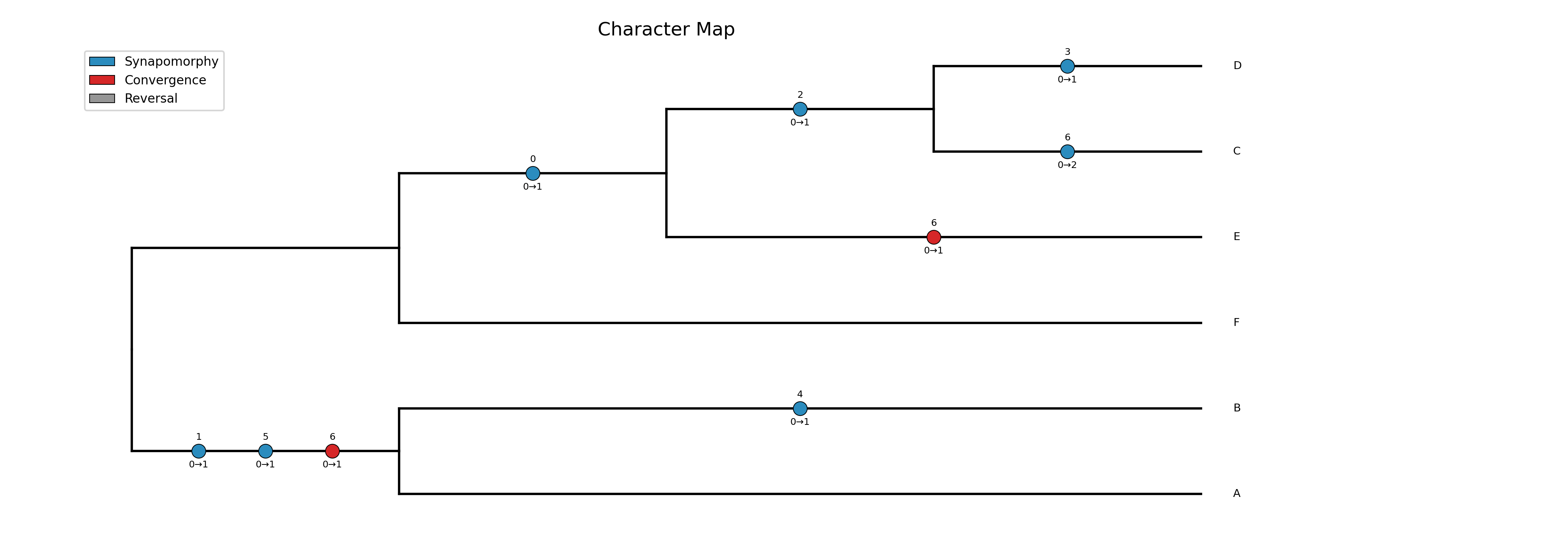
Map character state changes onto a phylogeny using Fitch parsimony with ACCTRAN (default) or DELTRAN optimization. Produces a cladogram (default) or phylogram with color-coded circles on each branch showing where character state changes occur. This is useful for visualizing synapomorphies and homoplasies in morphological datasets, similar to the classic Winclada software.
Each circle on a branch represents a character state change. The
number above the circle is the character index (matching the column
in the input matrix). The transition below shows the old and new
state (e.g., 0→1). Circle color indicates the type of change:
Blue circles: synapomorphies — this character changed to this state only once on the entire tree, uniquely supporting the clade
Red circles: convergences — this character independently gained the same state on two or more branches
Gray circles: reversals — the character returned to a state previously seen at an ancestor
Note that the same state transition (e.g., 0→1) may appear in
different colors because the color reflects how many times that
particular character underwent that transition across the tree, not the
state values themselves.
Input: a Newick tree file and a TSV character matrix (header row with
character names, one row per taxon with discrete states). Missing data
(? or -) is treated as a wildcard.
Reports the consistency index (CI), retention index (RI), and total tree length (parsimony steps). CI and RI cross-validated against R's phangorn.
Polytomies are automatically resolved by inserting zero-length branches.
Example usage:
# Basic usage with default ACCTRAN optimization and cladogram layout
phykit character_map -t species.tre -d morphology.tsv -o charmap.png

# Use DELTRAN optimization and ladderize the tree
phykit character_map -t species.tre -d morphology.tsv -o charmap.png \
    --optimization deltran --ladderize

# Show only specific characters of interest
phykit character_map -t species.tre -d morphology.tsv -o charmap.png \
    --characters 0,3,7,12

# Phylogram layout with JSON output
phykit character_map -t species.tre -d morphology.tsv -o charmap.png \
    --phylogram --json
Input format — the character matrix is a tab-separated file where the first row is a header with character names, and each subsequent row has a taxon name followed by the character states:
taxon        char0   char1   char2   char3
Taxon_A      0       1       0       2
Taxon_B      0       1       1       0
Taxon_C      1       0       0       2
Taxon_D      1       0       1       1
Full usage:
phykit character_map -t <tree> -d <data> -o <output>
    [--optimization acctran|deltran] [--phylogram]
    [--characters 0,1,3] [--verbose] [--json]
    [--fig-width <float>] [--fig-height <float>] [--dpi <int>] [--no-title] [--title <str>]
    [--legend-position <str>] [--ylabel-fontsize <float>] [--xlabel-fontsize <float>]
    [--title-fontsize <float>] [--axis-fontsize <float>] [--colors <str>] [--ladderize]
Options:
-t/--tree: tree file in Newick format (required)
-d/--data: TSV character matrix with header row (required)
-o/--output: output figure path (.png, .pdf, .svg) (required)
--optimization: ancestral state optimization: acctran (default) or deltran
--phylogram: draw phylogram instead of cladogram
--characters: comma-separated character indices to display (0-based; all characters are still used for CI/RI)
--verbose: print per-character detail
--colors: comma-separated colors for synapomorphy, convergence, reversal (default: blue, red, gray)
--ladderize: ladderize (sort) the tree before plotting
--cladogram: draw cladogram (equal branch lengths, tips aligned) instead of phylogram
--circular: draw circular (radial/fan) phylogram instead of rectangular
--color-file: color annotation file for tip labels, clade ranges, and branch colors (iTOL-inspired TSV format)
--json: optional argument to print results as JSON
R validation: Validated against phytools in R
(see tests/r_validation/validate_character_map.R).
Chronogram
Function names: chronogram; chrono; time_tree
Command line interface: pk_chronogram; pk_chrono; pk_time_tree
Plot a chronogram (time-calibrated phylogeny) with geological timescale bands. Requires an ultrametric (or approximately ultrametric) tree and the root age in millions of years (Ma).
Geological epoch, period, or era bands are drawn behind the tree as colored stripes based on the ICS 2024 International Chronostratigraphic Chart. A labeled timescale bar is displayed below the tree. The time axis runs from past (left) to present (right).
95% HPD confidence intervals are automatically detected and drawn
when the input tree contains BEAST (height_95%_HPD) or MCMCTree
(95%HPD) node annotations. The intervals appear as translucent
blue bars at each internal node — no extra flags needed. Trees without
annotations are plotted without bars.
The --timescale option controls the level of detail:
auto (default): selects epochs for trees <= 66 Ma, periods for <= 252 Ma, eras for deeper timescales
epoch: Cenozoic and Mesozoic epochs (Holocene through Early Triassic)
period: geological periods (Quaternary through Cambrian)
era: Cenozoic, Mesozoic, Paleozoic
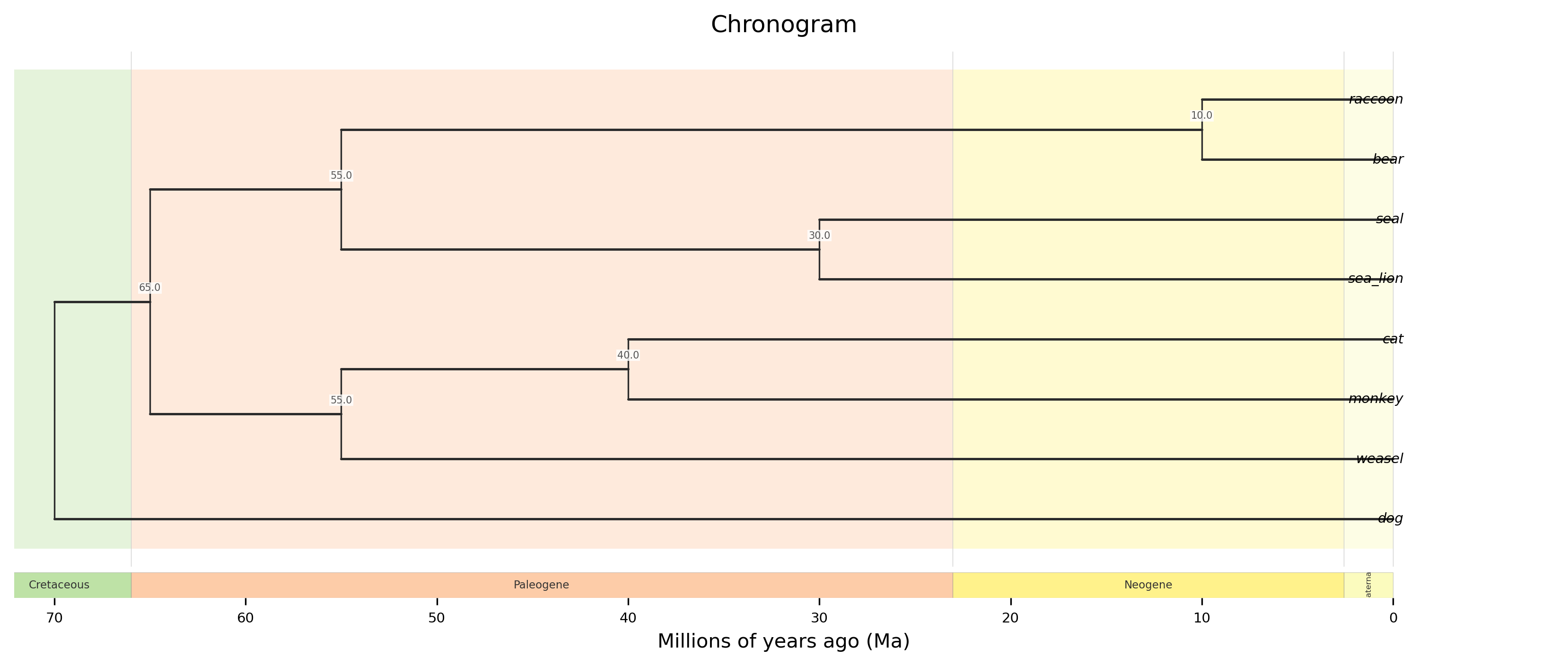
Rectangular chronogram with epoch bands, node age labels, and a geological timescale bar.
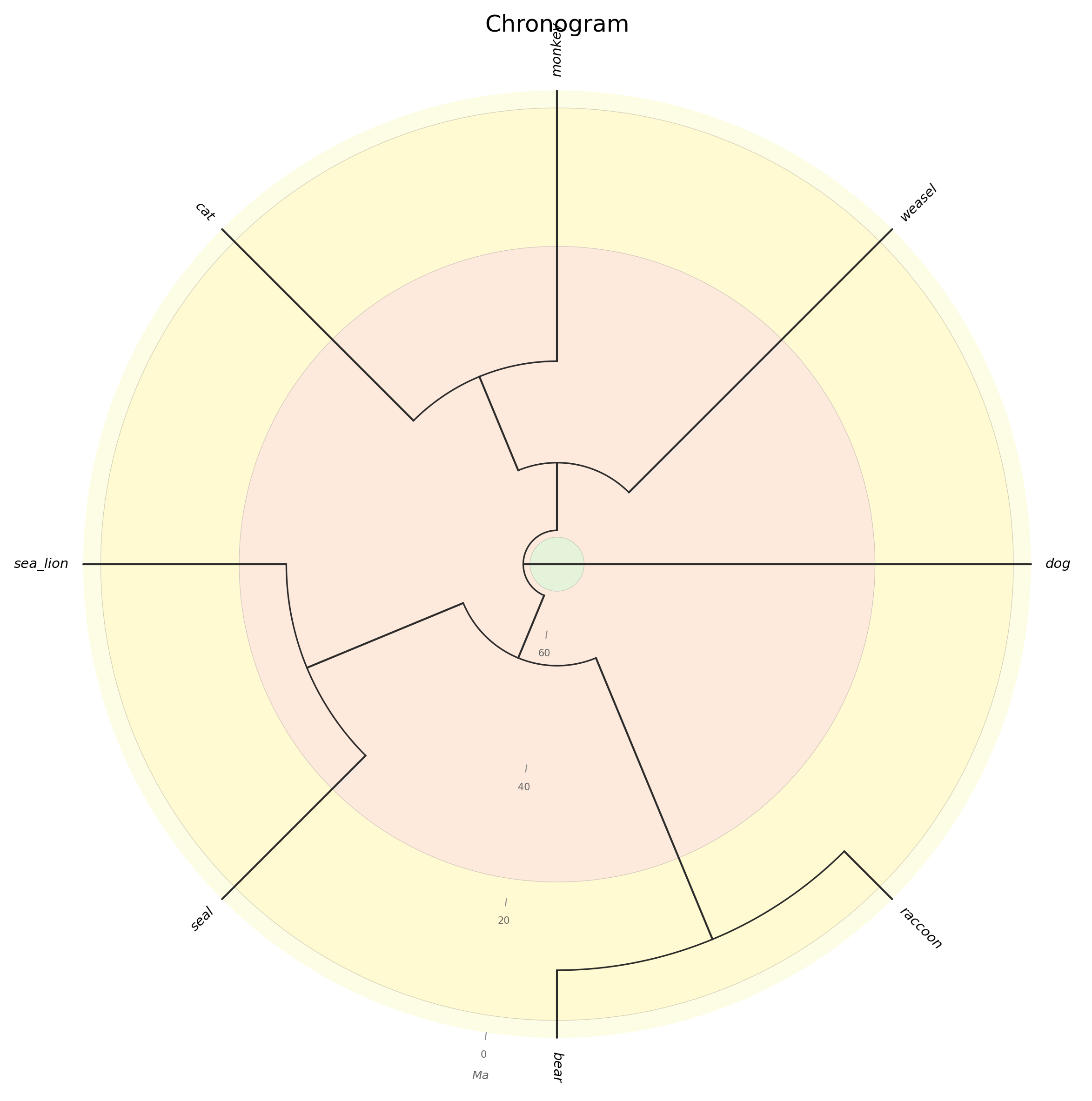
Circular chronogram with concentric geological epoch rings and radial time tick marks.
phykit chronogram -t <tree> --root-age <float> --plot-output <file>
    [--timescale auto|epoch|period|era] [--node-ages]
    [--circular] [--ladderize] [--color-file <file>] [--json]
Options:
-t/--tree: ultrametric tree file (required)
--root-age: age of the root in millions of years (Ma; required)
--plot-output: output figure path (.png, .pdf, .svg; required)
--timescale: timescale level — auto (default), epoch, period, or era
--node-ages: label internal nodes with divergence times (Ma)
--circular: draw circular chronogram with concentric geological rings
--ladderize: ladderize (sort) the tree before plotting
--color-file: color annotation file for tip labels, clade ranges, and branch colors (iTOL-inspired TSV format)
--json: output node ages as JSON
Collapse bipartitions
Function names: collapse_branches; collapse; cb
Command line interface: pk_collapse_branches; pk_collapse; pk_cb
Collapse branches on a phylogeny according to bipartition support.
Bipartitions will be collapsed if they are less than the user specified value.
phykit collapse_branches <tree> -s/--support n [-o/--output <output_file>] [--json]
Options:
<tree>: first argument after function name should be a tree file
-s/--support: bipartitions with support less than this value will be
collapsed
-o/--output: optional argument to name the outputted tree file. Default
output will have the same name as the input file but with the suffix
".collapsed_(support).tre"
--json: optional argument to print results as JSON
Concordance-aware ancestral state reconstruction
Function names: concordance_asr; conc_asr; casr
Command line interface: pk_concordance_asr; pk_conc_asr; pk_casr
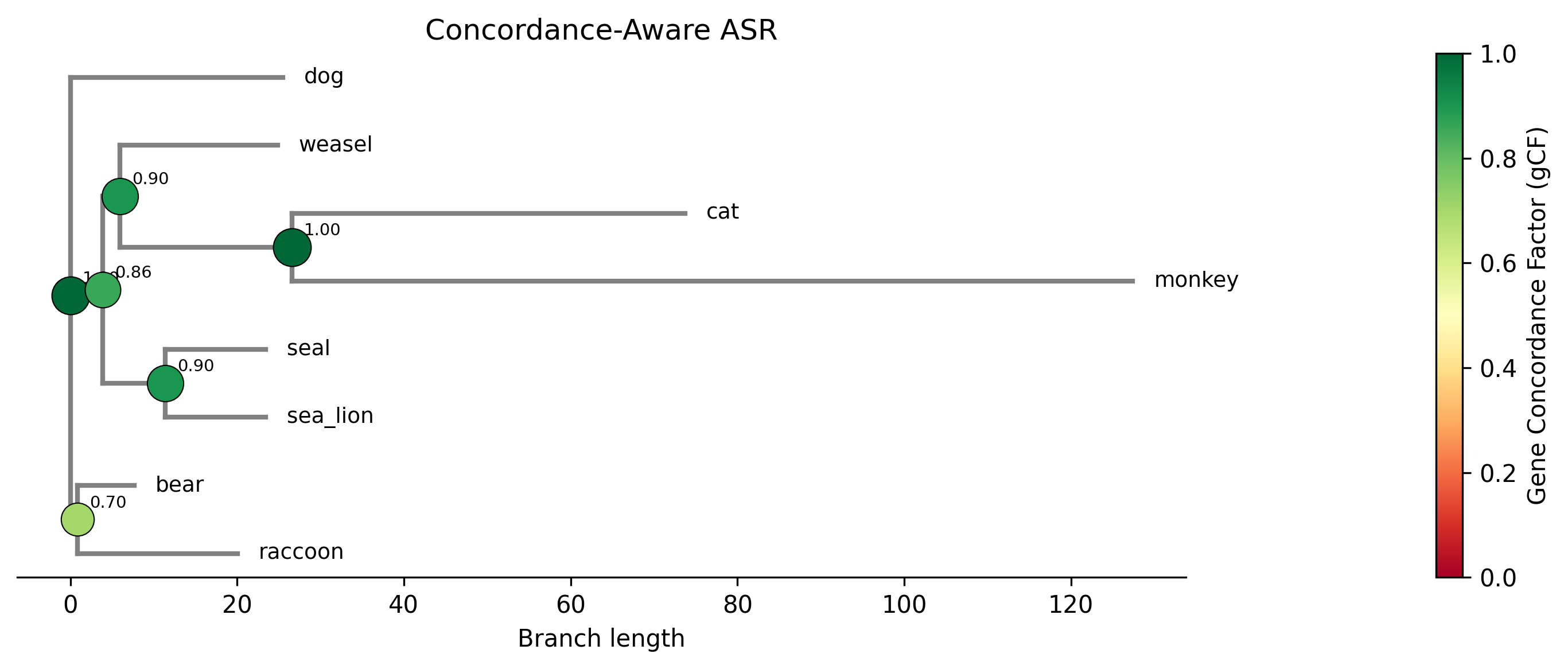
Concordance-aware ancestral state reconstruction that incorporates gene tree discordance into ancestral estimates. Standard ASR operates on a single species tree and ignores gene tree conflict. This command propagates topological uncertainty from gene tree discordance into ancestral state estimates using gene concordance factors (gCF).
Two strategies are available:
weighted (default): For each internal node, compute gCF (fraction of gene trees supporting the species-tree bipartition) and gDF1, gDF2 (fractions for NNI alternatives). Run ASR on the species tree and NNI alternative trees, then combine estimates weighted by concordance. Uses the law of total variance to separate topological vs parameter uncertainty.
distribution: Run ASR independently on each gene tree, map nodes across trees by descendant-set identity, and report concordance-weighted means with percentile confidence intervals (2.5th--97.5th).
phykit concordance_asr -t <species_tree> -g <gene_trees> -d <trait_data>
    [-c <trait>] [-m weighted|distribution] [--ci]
    [--plot <output>] [--plot-uncertainty <output>] [--missing-taxa error|shared]
    [--fig-width <float>] [--fig-height <float>] [--dpi <int>] [--no-title] [--title <str>]
    [--legend-position <str>] [--ylabel-fontsize <float>] [--xlabel-fontsize <float>]
    [--title-fontsize <float>] [--axis-fontsize <float>] [--colors <str>] [--ladderize] [--cladogram] [--circular] [--color-file <file>] [--json]
Options:
-t/--tree: species tree file
-g/--gene-trees: file with gene trees (multi-Newick, one per line)
-d/--trait_data: trait data file (two-column or multi-trait with header)
-c/--trait: trait column name (required for multi-trait files)
-m/--method: method to use: weighted or distribution (default: weighted)
--ci: include 95% confidence intervals
--plot: output path for concordance ASR contMap plot
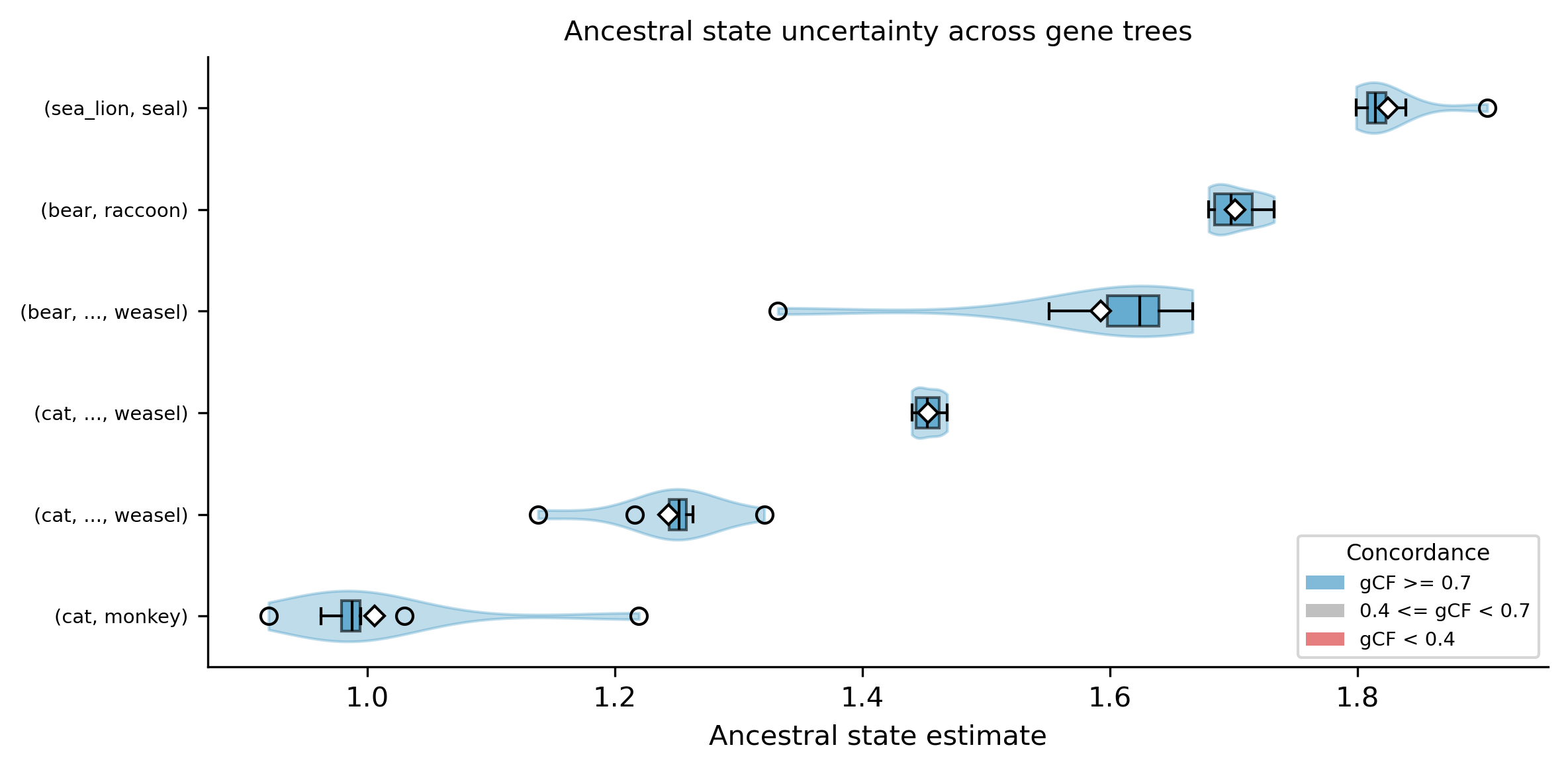
--plot-uncertainty: output path for uncertainty plot showing the distribution of ancestral estimates across gene trees (distribution method) or concordance sources (weighted method) as violin + boxplots colored by gCF
--missing-taxa: how to handle taxa mismatches: shared (default, prune to intersection) or error (reject)
--fig-width: figure width in inches (auto-scaled if omitted)
--fig-height: figure height in inches (auto-scaled if omitted)
--dpi: resolution in DPI (default: 300)
--no-title: hide the plot title
--title: custom title text
--legend-position: legend location (e.g., "upper right", "none" to hide)
--ylabel-fontsize: font size for y-axis labels; 0 to hide
--xlabel-fontsize: font size for x-axis labels; 0 to hide
--title-fontsize: font size for the title
--axis-fontsize: font size for axis labels
--colors: comma-separated colors (hex or named)
--ladderize: ladderize (sort) the tree before plotting
--cladogram: draw cladogram (equal branch lengths, tips aligned) instead of phylogram
--circular: draw circular (radial/fan) phylogram instead of rectangular
--color-file: color annotation file for tip labels, clade ranges, and branch colors (iTOL-inspired TSV format)
--json: output results as JSON
Example output:
Concordance-Aware Ancestral State Reconstruction

Method: weighted
Number of tips: 8
Number of gene trees: 10
Sigma-squared (BM rate): 0.043893

Ancestral estimates:
  Node          Desc    Estimate     gCF                  95% CI    Var_topo   Var_param
  N1 (root)        8      1.6447   1.000        [0.8937, 2.3957]    0.000000    0.146822
  N2               2      1.6881   0.700        [0.9529, 2.4234]    0.000569    0.140151
  N3               5      1.4878   0.857        [0.6727, 2.3028]    0.005878    0.167045
  N4               2      1.7682   0.900        [0.8987, 2.6378]    0.015002    0.181806
  N5               3      1.2674   0.900        [0.3663, 2.1684]    0.001044    0.210295
  N6               2      0.9895   1.000       [-0.5654, 2.5443]    0.000000    0.629294
Example plot generated with the --plot option. Internal nodes are sized
and colored by gene concordance factor (gCF):
The --plot-uncertainty option generates a violin + boxplot showing the
distribution of ancestral state estimates for each internal node. For the
distribution method, each violin shows per-gene-tree estimates. For the
weighted method, each violin shows the concordant and discordant source
estimates. Nodes are colored by gCF: blue (gCF >= 0.7, high concordance),
gray (0.4 <= gCF < 0.7), red (gCF < 0.4, high discordance). Wide violins
indicate high uncertainty — the ancestral estimate varies substantially
across gene trees, suggesting that gene tree conflict propagates into
trait estimates at that node.
Consensus network
Function names: consensus_network; consnet; splitnet; splits_network
Command line interface: pk_consensus_network; pk_consnet; pk_splitnet; pk_splits_network
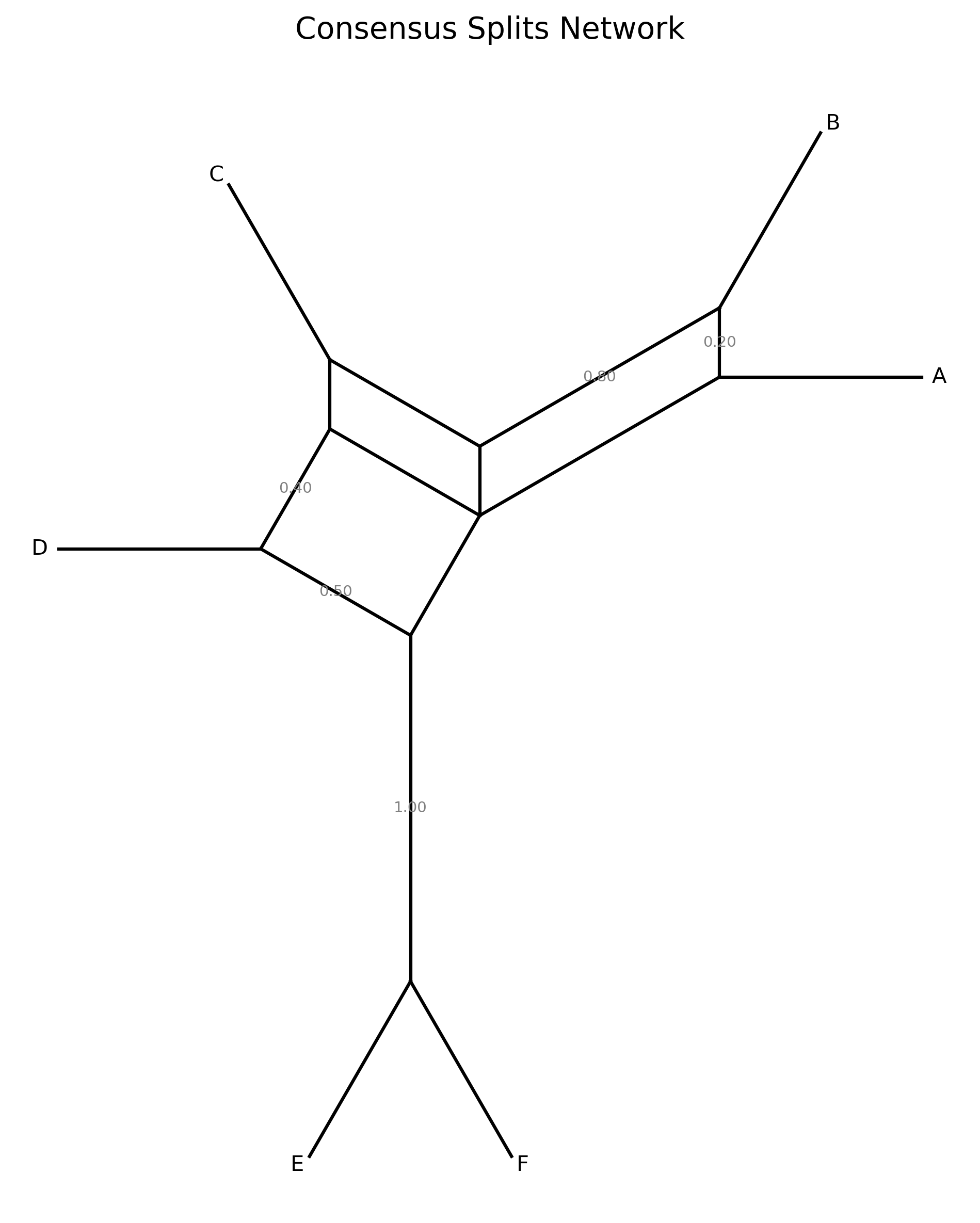
Extract bipartition splits from a collection of gene trees and summarize conflicting phylogenetic signal. Counts how frequently each non-trivial bipartition appears across input trees and filters by a minimum frequency threshold. Optionally draws a circular splits network diagram.
Polytomies (collapsed branches) in input trees are handled conservatively: splits from polytomous nodes are excluded since they represent unresolved relationships. Trifurcating roots (standard unrooted Newick) are not affected. This allows gene trees with collapsed low-support branches to be used directly as input.
Input can be either: 1) a file with one Newick tree per line, or 2) a file with one tree-file path per line.
phykit consensus_network -t/--trees <trees> [--threshold 0.1] [--missing-taxa error|shared] [--plot-output <file>]
    [--fig-width <float>] [--fig-height <float>] [--dpi <int>] [--no-title] [--title <str>]
    [--legend-position <str>] [--ylabel-fontsize <float>] [--xlabel-fontsize <float>]
    [--title-fontsize <float>] [--axis-fontsize <float>] [--colors <str>] [--ladderize] [--cladogram] [--circular] [--color-file <file>] [--json]
Options:
-t/--trees: file containing trees (one Newick per line) or tree-file paths (one per line)
--threshold: minimum split frequency to include, between 0 and 1 (default: 0.1)
--missing-taxa: handling strategy for mismatched taxa (error or shared; default: error)
--plot-output: output filename for the circular splits network plot (optional)
--fig-width: figure width in inches (auto-scaled if omitted)
--fig-height: figure height in inches (auto-scaled if omitted)
--dpi: resolution in DPI (default: 300)
--no-title: hide the plot title
--title: custom title text
--legend-position: legend location (e.g., "upper right", "none" to hide)
--ylabel-fontsize: font size for y-axis labels; 0 to hide
--xlabel-fontsize: font size for x-axis labels; 0 to hide
--title-fontsize: font size for the title
--axis-fontsize: font size for axis labels
--colors: comma-separated colors (hex or named)
--ladderize: ladderize (sort) the tree before plotting
--cladogram: draw cladogram (equal branch lengths, tips aligned) instead of phylogram
--circular: draw circular (radial/fan) phylogram instead of rectangular
--color-file: color annotation file for tip labels, clade ranges, and branch colors (iTOL-inspired TSV format)
--json: optional argument to print results as JSON
When --plot-output is specified, a circular splits network diagram is produced.
Taxa are arranged at equal angles around a circle. Each split is drawn as a chord
connecting the boundary points between the two sides of the bipartition. Chord
thickness and opacity scale with split frequency — thicker, darker lines indicate
splits supported by more gene trees.
Consensus tree
Function names: consensus_tree; consensus; ctree
Command line interface: pk_consensus_tree; pk_consensus; pk_ctree
Infer a consensus tree from a collection of trees.
Input can be either: 1) a file with one Newick tree per line, or 2) a file with one tree-file path per line.
Consensus methods:
* majority: majority-rule consensus (default)
* strict: strict consensus
Missing taxa handling:
* --missing-taxa error (default): exits if trees do not share identical tip sets
* --missing-taxa shared: prunes all trees to the intersection of taxa before inferring consensus
phykit consensus_tree -t/--trees <trees> [-m/--method strict|majority] [--missing-taxa error|shared] [--json]
Options:
-t/--trees: file containing trees (one Newick per line) or tree-file paths (one per line)
-m/--method: consensus method (strict or majority; default: majority)
--missing-taxa: handling strategy for mismatched taxa (error or shared; default: error)
--json: optional argument to print results as JSON
Continuous trait evolution model comparison (fitContinuous)
Function names: fit_continuous; fitcontinuous; fc
Command line interface: pk_fit_continuous; pk_fitcontinuous; pk_fc
Compare models of continuous trait evolution on a phylogeny, analogous to
R's geiger::fitContinuous(). Fits up to 7 models and ranks them by
AIC, BIC, and AIC weights.
Models:
BM -- Brownian motion (baseline, 2 params)
OU -- Ornstein-Uhlenbeck / stabilizing selection (3 params)
EB -- Early Burst (Harmon et al. 2010) (3 params)
Lambda -- Pagel's lambda / phylogenetic signal (3 params)
Delta -- Pagel's delta / tempo of evolution (3 params)
Kappa -- Pagel's kappa / punctuational vs gradual (3 params)
White -- White noise / no phylogenetic signal (2 params)
Each model reports R² = 1 - (σ²_model / σ²_White), measuring how much variance is explained relative to the white noise baseline. White serves as the reference (R² = 0).
phykit fit_continuous -t <tree> -d <trait_data> [--models BM,OU,Lambda] [-g <gene_trees>] [--json]
Options:
-t/--tree: a tree file in Newick format
-d/--trait_data: tab-delimited trait file (taxon<tab>value)
--models: comma-separated list of models to fit (default: all 7)
-g/--gene-trees: optional multi-Newick file of gene trees; when provided, uses a discordance-aware VCV (genome-wide average) instead of the species-tree VCV
--json: optional argument to print results as JSON
Example output:
Model Comparison (fitContinuous)

Number of tips: 8

Model       Param     Value      Sigma2    z0        LL         AIC     dAIC    AICw    BIC     dBIC
BM          -         -          0.0384    1.6447    -11.570    27.14   0.00    0.453   27.83   0.00
OU          alpha     0.0012     0.0385    1.6420    -11.568    29.14   2.00    0.167   30.18   2.35
...

Best model (AIC): BM
Best model (BIC): BM
R validation: Validated against geiger in R
(see tests/r_validation/validate_fit_continuous_r2.R).
Continuous trait mapping (contMap)
Function names: cont_map; contmap; cmap
Command line interface: pk_cont_map; pk_contmap; pk_cmap
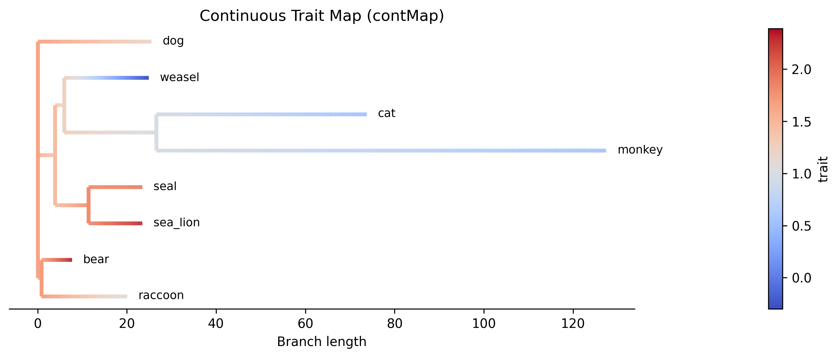
Plot a phylogram with branches colored by continuous trait values
(analogous to R's phytools::contMap()). Ancestral states are
estimated via maximum-likelihood (two-pass Felsenstein algorithm)
and mapped onto branches using a color gradient (coolwarm colormap).
phykit cont_map -t <tree> -d <trait_data> -o <output.png>
    [--fig-width <float>] [--fig-height <float>] [--dpi <int>] [--no-title] [--title <str>]
    [--legend-position <str>] [--ylabel-fontsize <float>] [--xlabel-fontsize <float>]
    [--title-fontsize <float>] [--axis-fontsize <float>] [--colors <str>] [--ladderize] [--cladogram] [--circular] [--color-file <file>] [--json]
Options:
-t/--tree: a tree file in Newick format
-d/--trait_data: tab-delimited trait file (taxon<tab>value)
-o/--output: output plot file path (required)
--fig-width: figure width in inches (auto-scaled if omitted)
--fig-height: figure height in inches (auto-scaled if omitted)
--dpi: resolution in DPI (default: 300)
--no-title: hide the plot title
--title: custom title text
--legend-position: legend location (e.g., "upper right", "none" to hide)
--ylabel-fontsize: font size for y-axis labels; 0 to hide
--xlabel-fontsize: font size for x-axis labels; 0 to hide
--title-fontsize: font size for the title
--axis-fontsize: font size for axis labels
--colors: comma-separated colors (hex or named)
--ladderize: ladderize (sort) the tree before plotting
--cladogram: draw cladogram (equal branch lengths, tips aligned) instead of phylogram
--circular: draw circular (radial/fan) phylogram instead of rectangular
--color-file: color annotation file for tip labels, clade ranges, and branch colors (iTOL-inspired TSV format)
--json: optional argument to print results as JSON
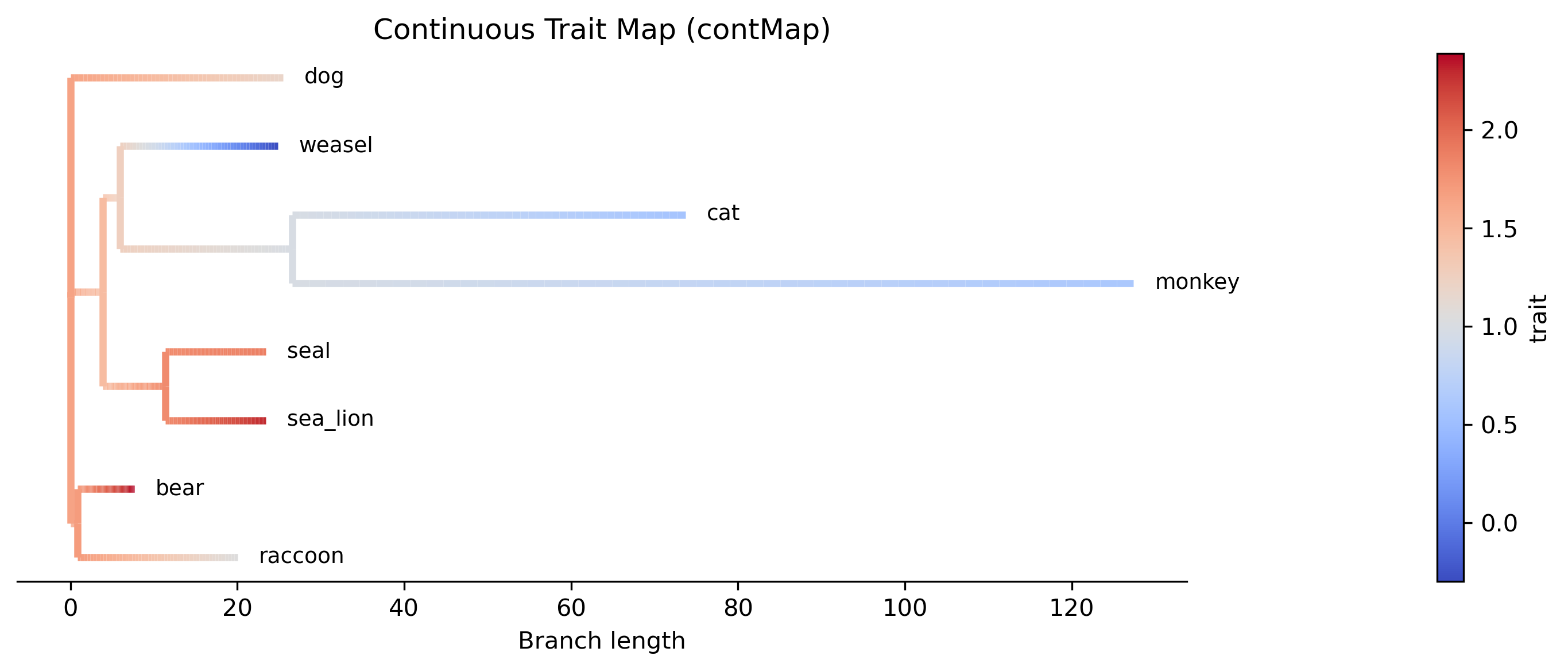
Cophylogenetic plot (tanglegram)
Function names: cophylo; tanglegram; tangle
Command line interface: pk_cophylo; pk_tanglegram; pk_tangle
Plot a cophylogenetic tanglegram of two phylogenies (analogous to R's
phytools::cophylo()). Draws two trees facing each other with
connecting lines between matching taxa. By default, taxa are matched
by identical tip names. Internal nodes of tree2 are rotated to minimize
line crossings.
phykit cophylo -t <tree1> -t2 <tree2> -o <output.png> [-m <mapping>]
    [--fig-width <float>] [--fig-height <float>] [--dpi <int>] [--no-title] [--title <str>]
    [--legend-position <str>] [--ylabel-fontsize <float>] [--xlabel-fontsize <float>]
    [--title-fontsize <float>] [--axis-fontsize <float>] [--colors <str>] [--ladderize] [--cladogram] [--circular] [--color-file <file>] [--json]
Options:
-t/--tree1: first tree file in Newick format
-t2/--tree2: second tree file in Newick format
-o/--output: output plot file path (required)
-m/--mapping: optional tab-delimited mapping file (taxon1<tab>taxon2)
--fig-width: figure width in inches (auto-scaled if omitted)
--fig-height: figure height in inches (auto-scaled if omitted)
--dpi: resolution in DPI (default: 300)
--no-title: hide the plot title
--title: custom title text
--legend-position: legend location (e.g., "upper right", "none" to hide)
--ylabel-fontsize: font size for y-axis labels; 0 to hide
--xlabel-fontsize: font size for x-axis labels; 0 to hide
--title-fontsize: font size for the title
--axis-fontsize: font size for axis labels
--colors: comma-separated colors (hex or named)
--ladderize: ladderize (sort) the tree before plotting
--cladogram: draw cladogram (equal branch lengths, tips aligned) instead of phylogram
--circular: draw circular (radial/fan) phylogram instead of rectangular
--color-file: color annotation file for tip labels, clade ranges, and branch colors (iTOL-inspired TSV format)
--json: optional argument to print results as JSON
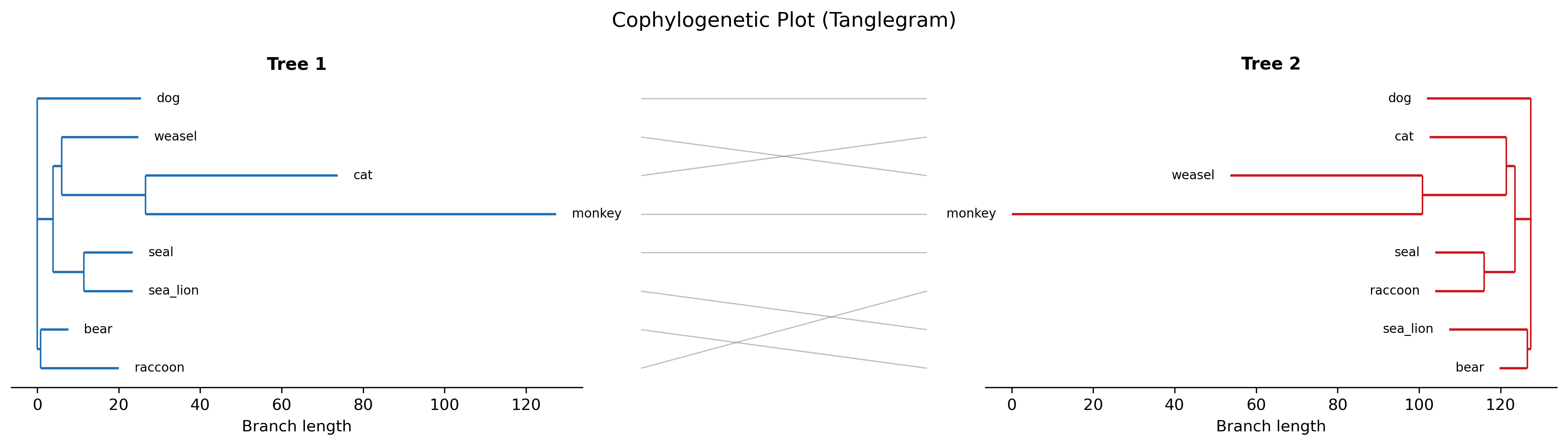
Covarying evolutionary rates
Function names: covarying_evolutionary_rates; cover
Command line interface: pk_covarying_evolutionary_rates; pk_cover
Determine if two genes have a signature of covariation with one another. Genes that have covarying evolutionary histories tend to have similar functions and expression levels.
Input two phylogenies and calculate the correlation among relative evolutionary rates between the two phylogenies. The two input trees do not have to have the same taxa. This function will first prune both trees to have the same tips. To transform branch lengths into relative rates, PhyKIT uses the putative species tree's branch lengths, which is input by the user. As recommended by the original method developers, outlier branch lengths are removed. Outlier branches have a relative evolutionary rate greater than five.
PhyKIT reports two tab delimited values: col1: correlation coefficient col2: p-value
Method is empirically evaluated by Clark et al., Genome Research (2012), doi: 10.1101/gr.132647.111. Normalization method using a species tree follows Sato et al., Bioinformatics (2005), doi: 10.1093/bioinformatics/bti564.
phykit covarying_evolutionary_rates <tree_file_zero> <tree_file_one> -r/--reference <reference_tree_file> [-v/--verbose] [--plot] [--plot-output <path>]
    [--fig-width <float>] [--fig-height <float>] [--dpi <int>] [--no-title] [--title <str>]
    [--legend-position <str>] [--ylabel-fontsize <float>] [--xlabel-fontsize <float>]
    [--title-fontsize <float>] [--axis-fontsize <float>] [--colors <str>] [--ladderize] [--cladogram] [--circular] [--color-file <file>] [--json]
Options:
<tree_file_zero>: first argument after function name should be a tree file
<tree_file_one>: second argument after function name should be a tree file
-r/--reference: a tree to correct branch lengths by in the two input trees. Typically,
this is a putative species tree.
-v/--verbose: print out corrected branch lengths shared between tree 0 and tree 1
--plot: save a covarying-rates scatter plot
--plot-output: output path for plot (default: covarying_rates_plot.png)
--fig-width: figure width in inches (auto-scaled if omitted)
--fig-height: figure height in inches (auto-scaled if omitted)
--dpi: resolution in DPI (default: 300)
--no-title: hide the plot title
--title: custom title text
--legend-position: legend location (e.g., "upper right", "none" to hide)
--ylabel-fontsize: font size for y-axis labels; 0 to hide
--xlabel-fontsize: font size for x-axis labels; 0 to hide
--title-fontsize: font size for the title
--axis-fontsize: font size for axis labels
--colors: comma-separated colors (hex or named)
--ladderize: ladderize (sort) the tree before plotting
--cladogram: draw cladogram (equal branch lengths, tips aligned) instead of phylogram
--circular: draw circular (radial/fan) phylogram instead of rectangular
--color-file: color annotation file for tip labels, clade ranges, and branch colors (iTOL-inspired TSV format)
--json: optional argument to print results as JSON
D-statistic (ABBA-BABA test)
Function names: dstatistic; dstat; abba_baba
Command line interface: pk_dstatistic; pk_dstat; pk_abba_baba
Compute Patterson's D-statistic (ABBA-BABA test) for detecting
introgression or gene flow between taxa. Given a four-taxon alignment
with topology (((P1, P2), P3), Outgroup), the test counts ABBA
and BABA site patterns:
ABBA: P1 has the ancestral allele, P2 and P3 share the derived allele — suggests introgression between P2 and P3
BABA: P2 has the ancestral allele, P1 and P3 share the derived allele — suggests introgression between P1 and P3
D = (ABBA - BABA) / (ABBA + BABA): D = 0 under ILS alone; D significantly different from 0 indicates introgression
Note: the D-statistic identifies which pair of lineages exchanged genetic material but cannot determine the direction of gene flow within that pair.
Significance is assessed via block jackknife (Green et al. 2010), producing a Z-score and p-value.
Two input modes are supported:
Site patterns (
-a): counts ABBA/BABA from a FASTA alignment. Only biallelic sites with no gaps or ambiguous characters are considered. Significance via block jackknife.Gene trees (
-g): counts discordant quartet topologies from gene trees. Gene trees can have any number of taxa; only the quartet induced by the four specified taxa is evaluated. Significance via chi-squared test.
# Site-pattern mode
phykit dstatistic -a <alignment> --p1 <taxon> --p2 <taxon> --p3 <taxon> \
    --outgroup <taxon> [--block-size 100] [--json]

# Gene-tree mode
phykit dstatistic -g <gene_trees> --p1 <taxon> --p2 <taxon> --p3 <taxon> \
    --outgroup <taxon> [--json]
Options:
-a/--alignment: FASTA alignment file (site-pattern mode)
-g/--gene-trees: gene trees file, one Newick per line (gene-tree mode; trees can have any number of taxa)
--p1: taxon name for P1, sister to P2 (required)
--p2: taxon name for P2, sister to P1, potential recipient of gene flow from P3 (required)
--p3: taxon name for P3, donor lineage (required)
--outgroup: outgroup taxon name, determines ancestral allele (required)
--block-size: block size in sites for jackknife standard error estimation (default: 100; alignment mode only)
--support: minimum branch support threshold; gene tree branches below this value are collapsed and treated as unresolved (gene-tree mode only)
--json: optional argument to print results as JSON
Degree of violation of the molecular clock
Function names: degree_of_violation_of_a_molecular_clock; dvmc
Command line interface: pk_degree_of_violation_of_a_molecular_clock; pk_dvmc
Calculate degree of violation of a molecular clock (or DVMC) in a phylogeny.
Lower DVMC values are thought to be desirable because they are indicative of a lower degree of violation in the molecular clock assumption.
Typically, outgroup taxa are not included in molecular clock analysis. Thus, prior to calculating DVMC from a single gene tree, users may want to prune outgroup taxa from the phylogeny. To prune tips from a phylogeny, see the prune_tree function.
Calculate DVMC in a tree following Liu et al., PNAS (2017), doi: 10.1073/pnas.1616744114.
phykit degree_of_violation_of_a_molecular_clock <tree> [--json]
Options:
<tree>: input file tree name
--json: optional argument to print results as JSON
Density map
Function names: density_map; densitymap; dmap
Command line interface: pk_density_map; pk_densitymap; pk_dmap
Plot a phylogram with branches colored by posterior probabilities of
discrete character states from stochastic character mapping (analogous
to R's phytools::densityMap()). Runs N simulations of stochastic
character mapping internally and, for each point along each branch,
computes the fraction of simulations in each state.
phykit density_map -t <tree> -d <trait_data> -c <trait_column> -o <output.png> [-n <nsim>] [--seed <seed>]
    [--fig-width <float>] [--fig-height <float>] [--dpi <int>] [--no-title] [--title <str>]
    [--legend-position <str>] [--ylabel-fontsize <float>] [--xlabel-fontsize <float>]
    [--title-fontsize <float>] [--axis-fontsize <float>] [--colors <str>] [--ladderize] [--cladogram] [--circular] [--color-file <file>] [--json]
Options:
-t/--tree: a tree file in Newick format
-d/--trait_data: tab-delimited trait file (taxon<tab>state)
-c/--trait: column name of the trait to map
-o/--output: output plot file path (required)
-n/--nsim: number of stochastic mapping simulations (default: 100)
--seed: random seed for reproducibility
--fig-width: figure width in inches (auto-scaled if omitted)
--fig-height: figure height in inches (auto-scaled if omitted)
--dpi: resolution in DPI (default: 300)
--no-title: hide the plot title
--title: custom title text
--legend-position: legend location (e.g., "upper right", "none" to hide)
--ylabel-fontsize: font size for y-axis labels; 0 to hide
--xlabel-fontsize: font size for x-axis labels; 0 to hide
--title-fontsize: font size for the title
--axis-fontsize: font size for axis labels
--colors: comma-separated colors (hex or named)
--ladderize: ladderize (sort) the tree before plotting
--cladogram: draw cladogram (equal branch lengths, tips aligned) instead of phylogram
--circular: draw circular (radial/fan) phylogram instead of rectangular
--color-file: color annotation file for tip labels, clade ranges, and branch colors (iTOL-inspired TSV format)
--json: optional argument to print results as JSON
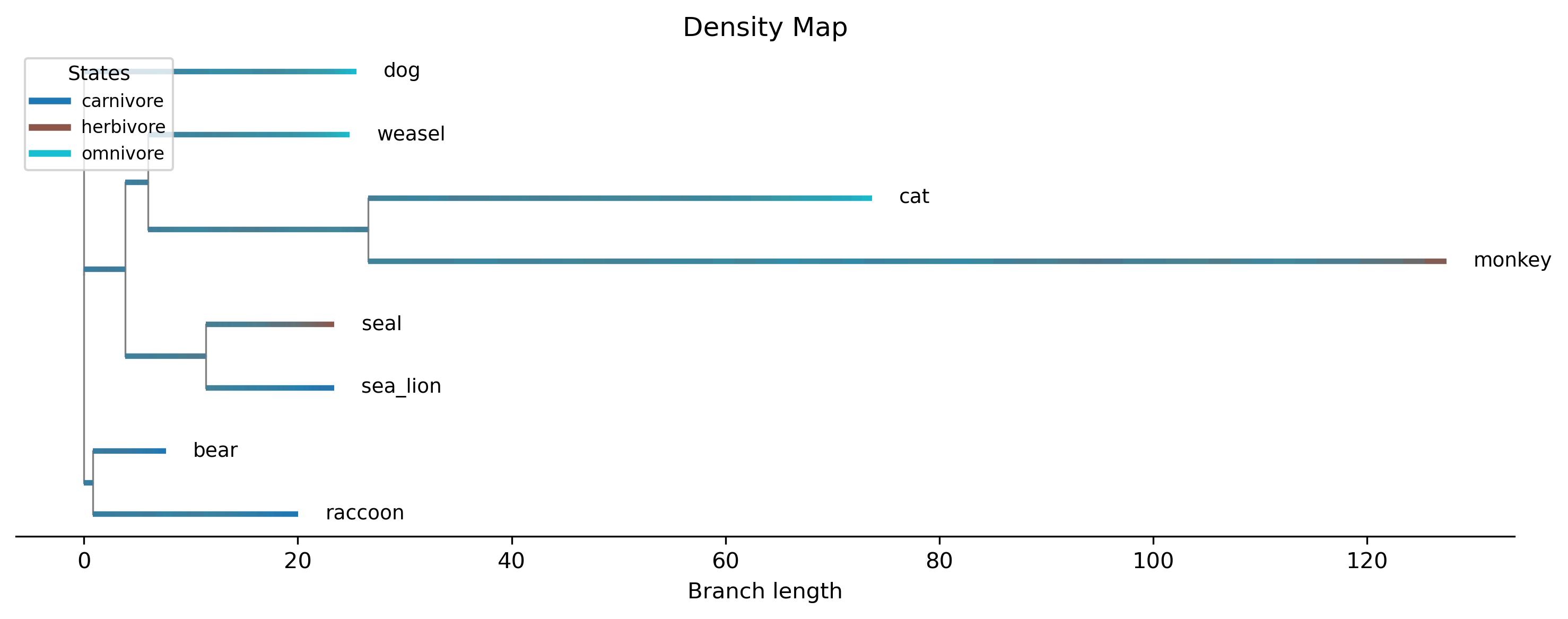
DFOIL test (Pease & Hahn 2015)
Function names: dfoil; dfoil_test
Command line interface: pk_dfoil; pk_dfoil_test
Compute DFOIL statistics (Pease & Hahn 2015) for detecting and polarizing
introgression in a 5-taxon symmetric phylogeny with topology
((P1, P2), (P3, P4), Outgroup).
P1 and P2 are sister taxa; P3 and P4 are sister taxa; the two pairs are sister to each other, with an outgroup rooting the tree.
Four D-statistics are computed: DFO (far-outer), DIL (inner-left), DFI (far-inner), and DOL (outer-left). Each is tested for significance using a chi-squared test (1 df). The sign pattern of the four statistics maps to a specific introgression scenario via the lookup table from Pease & Hahn (2015).
phykit dfoil -a <alignment> --p1 <taxon> --p2 <taxon> --p3 <taxon> \
    --p4 <taxon> --outgroup <taxon> [--json]
Options:
-a/--alignment: FASTA alignment file (required)
--p1: taxon name for P1, sister to P2 (required)
--p2: taxon name for P2, sister to P1 (required)
--p3: taxon name for P3, sister to P4 (required)
--p4: taxon name for P4, sister to P3 (required)
--outgroup: outgroup taxon name (required)
--json: optional argument to print results as JSON
Discordance asymmetry
Function names: discordance_asymmetry; disc_asym; da
Command line interface: pk_discordance_asymmetry; pk_disc_asym; pk_da
Test whether the two discordant NNI alternative topologies at each species tree branch are equally frequent. Under incomplete lineage sorting (ILS) alone, the two minor NNI alternatives (gDF1 and gDF2) should appear at equal frequency. When they are significantly asymmetric, it suggests introgression or gene flow between specific lineages.
For each internal branch of the species tree, a two-sided binomial test (H0: P(alt1) = 0.5) is applied, and p-values are corrected for multiple testing using Benjamini-Hochberg FDR.
Interpreting the plot: When --plot is used, branches are colored by
the asymmetry ratio = max(gDF1, gDF2) / (gDF1 + gDF2):
Blue/cool colors (ratio ~ 0.5): The two discordant topologies are roughly equal, consistent with ILS alone — no evidence of gene flow.
Red/warm colors (ratio → 1.0): One discordant topology is much more frequent than the other, suggesting introgression or gene flow.
Red stars: Branches where the asymmetry is statistically significant (FDR < 0.05) — these are introgression candidates.
Use --annotate to display gCF values on each branch. Use
--ylabel-fontsize 0 to hide tip labels for large trees, and
--legend-position none to hide both the legend and colorbar.
phykit discordance_asymmetry -t <species_tree> -g <gene_trees> [--plot <output>] [-v]
    [--annotate]
    [--fig-width <float>] [--fig-height <float>] [--dpi <int>] [--no-title] [--title <str>]
    [--legend-position <str>] [--ylabel-fontsize <float>] [--xlabel-fontsize <float>]
    [--title-fontsize <float>] [--axis-fontsize <float>] [--colors <str>] [--ladderize] [--cladogram] [--circular] [--color-file <file>] [--json]
Options:
-t/--tree: a species tree file
-g/--gene-trees: multi-Newick file of gene trees (branch lengths not required)
--plot: optional output path for asymmetry phylogram (PNG)
-v/--verbose: print per-branch details
--fig-width: figure width in inches (auto-scaled if omitted)
--fig-height: figure height in inches (auto-scaled if omitted)
--dpi: resolution in DPI (default: 300)
--no-title: hide the plot title
--title: custom title text
--legend-position: legend location (e.g., "upper right", "none" to hide)
--ylabel-fontsize: font size for y-axis labels; 0 to hide
--xlabel-fontsize: font size for x-axis labels; 0 to hide
--title-fontsize: font size for the title
--axis-fontsize: font size for axis labels
--colors: comma-separated colors (hex or named)
--ladderize: ladderize (sort) the tree before plotting
--cladogram: draw cladogram (equal branch lengths, tips aligned) instead of phylogram
--circular: draw circular (radial/fan) phylogram instead of rectangular
--color-file: color annotation file for tip labels, clade ranges, and branch colors (iTOL-inspired TSV format)
--json: optional argument to print results as JSON
Example output:
branch                          n_conc  n_alt1  n_alt2  asym_ratio     binom_p       fdr_p   gene_flow
------------------------------------------------------------------------------------------------------
bear,dog,raccoon                     6       0       1       1.000      1.0000      1.0000           -
bear,raccoon                         7       1       2       0.667      1.0000      1.0000           -
cat,monkey                          10       0       0          NA          NA          NA           -
cat,monkey,weasel                    9       1       0       1.000      1.0000      1.0000           -
sea_lion,seal                        9       1       0       1.000      1.0000      1.0000           -
---
Summary: 4 branches tested, 0 significant (FDR<0.05)
Each row corresponds to an internal branch of the species tree identified by the
smaller partition of taxa. The n_conc column shows concordant gene trees, while
n_alt1 and n_alt2 show the counts for the two NNI alternative topologies.
The asym_ratio is max(n_alt1, n_alt2) / (n_alt1 + n_alt2), ranging from 0.5
(perfectly symmetric) to 1.0 (maximally asymmetric). NA indicates no discordant
gene trees were observed. The binom_p is the two-sided binomial test p-value,
fdr_p is the Benjamini-Hochberg corrected p-value, and gene_flow shows
which NNI alternative is favored when the result is significant (FDR < 0.05).
Interpretation:
Symmetric discordance (asym_ratio near 0.5, not significant): Consistent with ILS alone — both NNI alternatives arise with equal frequency from random coalescent sorting.
Asymmetric discordance (asym_ratio near 1.0, significant): Suggests gene flow or introgression. The favored NNI alternative indicates which lineages are exchanging genetic material. For alt1, gene flow is between the C1 lineage and the S (sibling) lineage; for alt2, gene flow is between C2 and S.
To generate a visualization:
phykit discordance_asymmetry -t <species_tree> -g <gene_trees> --plot asymmetry.png
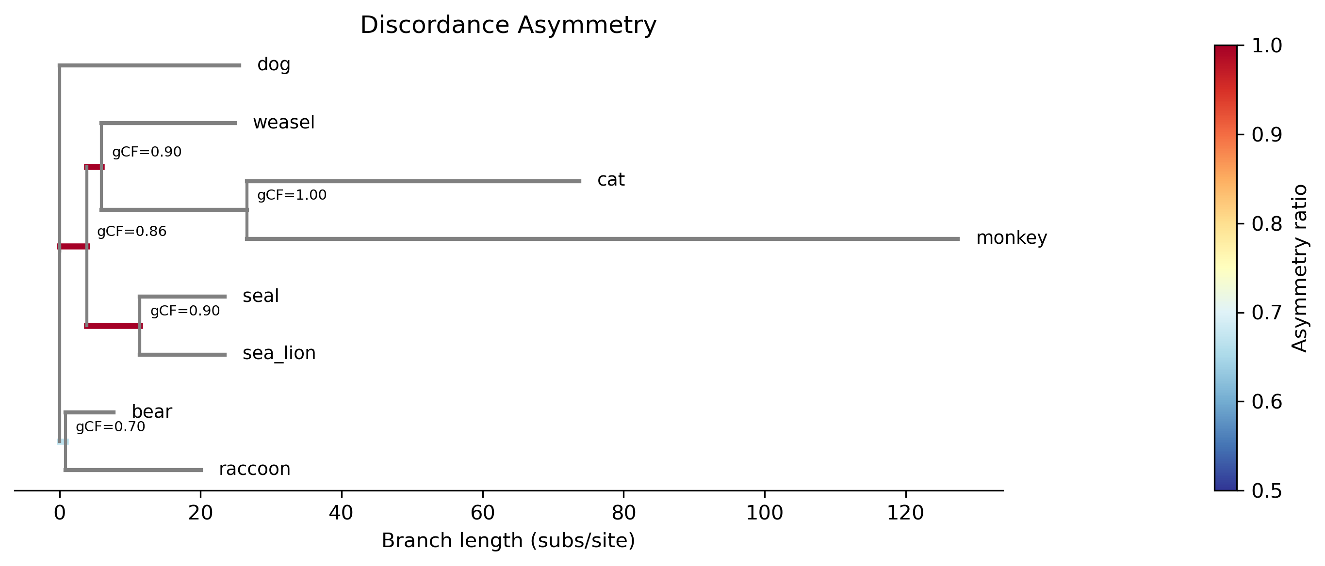
The plot shows a phylogram with internal branches colored by asymmetry ratio using a diverging colormap (blue = symmetric/0.5, red = highly asymmetric/1.0). Significant branches (FDR < 0.05) are marked with a red star. Internal nodes are annotated with gCF values.
Discrete trait evolution model comparison (fitDiscrete)
Function names: fit_discrete; fitdiscrete; fd
Command line interface: pk_fit_discrete; pk_fitdiscrete; pk_fd
Compare models of discrete trait evolution on a phylogeny. Fits ER (Equal Rates), SYM (Symmetric), and ARD (All Rates Different) Mk models of discrete character evolution via maximum likelihood. Compares models using AIC and BIC.
Analogous to R's geiger::fitDiscrete(). Cross-validated against R's geiger package.
phykit fit_discrete -t <tree> -d <trait_data> -c <trait>
        [--models ER,SYM,ARD] [--json]
Options:
-t/--tree: tree file (required)
-d/--trait_data: trait data file in TSV format (required)
-c/--trait: column name for the discrete trait in the data file (required)
--models: comma-separated list of models to fit (default: ER,SYM,ARD)
--json: optional argument to print results as JSON
R validation: Validated against geiger in R
(see tests/r_validation/validate_fit_discrete.R).
Disparity through time (DTT)
Function names: dtt; disparity_through_time
Command line interface: pk_dtt; pk_disparity_through_time
Compute disparity-through-time (DTT) curves following Harmon et al. (2003). At each branching time the mean relative subclade disparity is calculated. Under Brownian motion the DTT curve declines linearly from 1 to 0; deviations from this expectation reveal tempo of morphological diversification.
The Morphological Disparity Index (MDI) measures the area between the observed DTT and the Brownian motion null median. Positive MDI indicates late disparity accumulation; negative MDI indicates early disparity accumulation (consistent with adaptive radiation).
phykit dtt -t <tree> --traits <traits_file>
    [--trait <column>] [--index avg_sq|avg_manhattan]
    [--nsim <int>] [--seed <int>]
    [--plot-output <file>] [--json]
    [--fig-width <float>] [--fig-height <float>] [--dpi <int>] [--no-title] [--title <str>]
    [--legend-position <str>] [--ylabel-fontsize <float>] [--xlabel-fontsize <float>]
    [--title-fontsize <float>] [--axis-fontsize <float>] [--colors <str>] [--ladderize] [--cladogram] [--circular] [--color-file <file>]
Options:
-t/--tree: ultrametric tree file (required)
--traits: TSV file with header row; first column taxon, remaining columns are trait values (required)
--trait: specific trait column name; if omitted all trait columns are used (multivariate DTT)
--index: disparity index — avg_sq (average squared Euclidean distance, default) or avg_manhattan
--nsim: number of Brownian motion simulations for null DTT envelope and MDI p-value (default: 0, no simulations)
--seed: random seed for reproducibility
--plot-output: output filename for the DTT plot (PNG, PDF, SVG)
--json: output results as JSON
Default output: text summary with DTT curve data points.
# Single trait DTT
phykit dtt -t species.tre --traits traits.tsv --trait body_mass

# Multivariate DTT (all traits)
phykit dtt -t species.tre --traits traits.tsv

# With BM null envelope and MDI p-value
phykit dtt -t species.tre --traits traits.tsv --trait body_mass --nsim 1000 --seed 42

# With plot output
phykit dtt -t species.tre --traits traits.tsv --trait body_mass --nsim 1000 --plot-output dtt.png

# JSON output
phykit dtt -t species.tre --traits traits.tsv --trait body_mass --json
R validation: Validated against geiger::dtt() in R
(see tests/r_validation/validate_dtt.R).
Evolutionary rate
Function names: evolutionary_rate; evo_rate
Command line interface: pk_evolutionary_rate; pk_evo_rate
Calculate a tree-based estimation of the evolutionary rate of a gene.
Evolutionary rate is the total tree length divided by the number of terminals.
Calculate evolutionary rate following Telford et al., Proceedings of the Royal Society B (2014).
phykit evolutionary_rate <tree> [--json]
Options:
<tree>: input file tree name
--json: optional argument to print results as JSON
Evolutionary tempo mapping
Function names: evo_tempo_map; etm
Command line interface: pk_evo_tempo_map; pk_etm
Detect rate-topology associations by comparing branch length distributions between concordant and discordant gene trees at each species tree branch.
Under the multispecies coalescent, discordant gene trees should have shorter internal branches near the discordant node (because the coalescence happened deeper, in the ancestral population). Deviations from this expectation suggest substitution rate heterogeneity correlated with topology, which could indicate adaptive evolution, different selective pressures in hybridizing lineages, or systematic error from model misspecification.
For each internal branch of the species tree, gene trees are classified as concordant or discordant via bipartition matching (same as gCF). The homologous branch length is extracted from each gene tree and the two groups are compared using a Mann-Whitney U test and a permutation test (1000 permutations). P-values are corrected for multiple testing using Benjamini-Hochberg FDR.
A global treeness (internal/total branch length ratio) comparison between concordant and discordant gene trees is also reported.
phykit evo_tempo_map -t <species_tree> -g <gene_trees> [--plot <output>] [-v]
    [--fig-width <float>] [--fig-height <float>] [--dpi <int>] [--no-title] [--title <str>]
    [--legend-position <str>] [--ylabel-fontsize <float>] [--xlabel-fontsize <float>]
    [--title-fontsize <float>] [--axis-fontsize <float>] [--colors <str>] [--ladderize] [--cladogram] [--circular] [--color-file <file>] [--json]
Options:
-t/--tree: a species tree file
-g/--gene-trees: multi-Newick file of gene trees with branch lengths
--plot: optional output path for box/strip plot (PNG)
-v/--verbose: print per-gene-tree classification details
--fig-width: figure width in inches (auto-scaled if omitted)
--fig-height: figure height in inches (auto-scaled if omitted)
--dpi: resolution in DPI (default: 300)
--no-title: hide the plot title
--title: custom title text
--legend-position: legend location (e.g., "upper right", "none" to hide)
--ylabel-fontsize: font size for y-axis labels; 0 to hide
--xlabel-fontsize: font size for x-axis labels; 0 to hide
--title-fontsize: font size for the title
--axis-fontsize: font size for axis labels
--colors: comma-separated colors (hex or named)
--ladderize: ladderize (sort) the tree before plotting
--cladogram: draw cladogram (equal branch lengths, tips aligned) instead of phylogram
--circular: draw circular (radial/fan) phylogram instead of rectangular
--color-file: color annotation file for tip labels, clade ranges, and branch colors (iTOL-inspired TSV format)
--json: optional argument to print results as JSON
Example output:
branch                          n_conc  n_disc    med_conc    med_disc      U_pval   perm_pval       fdr_p
----------------------------------------------------------------------------------------------------------
bear,dog,raccoon                     6       1    3.875000    3.600000          NA          NA          NA
bear,raccoon                         7       3    0.880000    0.700000    0.516667    0.077000    0.516667
cat,monkey                          10       0   20.450000          NA          NA          NA          NA
cat,monkey,weasel                    9       1    2.120000    2.800000          NA          NA          NA
sea_lion,seal                        9       1    7.500000    7.200000          NA          NA          NA
---
Global treeness: concordant=0.126489 (n=6), discordant=0.119014 (n=4)
Branches tested: 1, significant (FDR<0.05): 0
Each row corresponds to an internal branch of the species tree identified by the
smaller partition of taxa. The n_conc and n_disc columns show how many gene
trees are concordant or discordant at that branch. The med_conc and med_disc
columns show the median branch length (in substitutions/site) for each group. The
U_pval is the two-sided Mann-Whitney U test p-value, perm_pval is the
permutation test p-value (1000 permutations), and fdr_p is the
Benjamini-Hochberg corrected p-value. Branches with fewer than 2 gene trees
in either group show NA for p-values.
The global treeness comparison tests whether concordant gene trees have systematically different ratios of internal to total branch lengths.
To generate a visualization:
phykit evo_tempo_map -t <species_tree> -g <gene_trees> --plot tempo_map.png
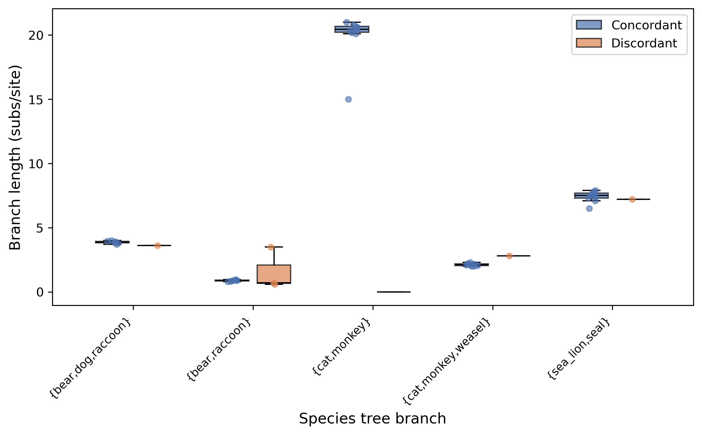
The plot shows grouped box plots with jittered data points for each species tree branch, comparing branch lengths between concordant (blue) and discordant (orange) gene trees. Branches where the FDR-corrected p-value is below 0.05 are marked with an asterisk.
Faith's phylogenetic diversity
Function names: faiths_pd; faith_pd; fpd; phylo_diversity
Command line interface: pk_faiths_pd; pk_faith_pd; pk_fpd; pk_phylo_diversity
Calculate Faith's phylogenetic diversity (PD) for a community of tips on a phylogeny (Faith, Biological Conservation, 1992; doi: 10.1016/0006-3207(92)91201-3).
Faith's PD is the sum of branch lengths in the minimum subtree that
connects a set of taxa. By default, the path from the community's most
recent common ancestor up to the tree root is included, matching the
original definition and picante::pd(..., include.root = TRUE). Pass
--exclude-root to sum only the branches of the induced subtree
rooted at the MRCA, matching picante::pd(..., include.root = FALSE).
The community is supplied as a single-column text file of tip labels, one per line.
phykit faiths_pd <tree> -t/--taxa <taxa_file> [--exclude-root] [--json]
Options:
<tree>: first argument after function name should be a tree file
-t/--taxa: file with one tip label per line defining the community
--exclude-root: sum only branches of the induced subtree rooted at the community MRCA
--json: optional argument to print results as JSON
Hybridization analysis
Function names: hybridization; hybrid; reticulation
Command line interface: pk_hybridization; pk_hybrid; pk_reticulation
Estimate the minimum number of reticulation events and localize where hybridization likely occurred on a species tree. For each internal branch, tests whether the two discordant NNI topologies are significantly asymmetric (binomial test with FDR correction). Asymmetric discordance suggests introgression/gene flow rather than ILS.
Each branch receives:
p-value: binomial test of gDF1 vs gDF2 equality (H0: ILS alone)
FDR-corrected p-value: Benjamini-Hochberg correction across all branches
Hybridization score: asymmetry ratio (0.5 = no signal, 1.0 = strong signal) for significant branches; 0 for non-significant
Favored alternative: which NNI topology is in excess, identifying which pair of lineages likely exchanged genes (but not the direction of gene flow)
The estimated reticulation count is the number of branches with significant
asymmetric discordance. Gene tree uncertainty can be accounted for with
--support to collapse low-support branches before topology determination.
phykit hybridization -t <species_tree> -g <gene_trees>
    [--support <float>] [--alpha 0.05] [--plot <output>] [--json]
    [--fig-width <float>] [--fig-height <float>] [--dpi <int>]
    [--ladderize] [--cladogram] [--circular] [--ylabel-fontsize <float>]
Options:
-t/--tree: species tree file (required)
-g/--gene-trees: gene trees file, one Newick per line (required)
--support: collapse gene tree branches below this support value before analysis
--alpha: FDR significance threshold (default: 0.05)
--plot: output hybridization score phylogram (branches colored by score, stars at significant nodes)
--json: optional argument to print results as JSON
Independent contrasts (PIC)
Function names: independent_contrasts; pic; phylo_contrasts
Command line interface: pk_independent_contrasts; pk_pic; pk_phylo_contrasts
Compute Felsenstein's (1985) phylogenetically independent contrasts for a continuous trait on a phylogeny. Each internal node yields one standardized contrast, producing n-1 contrasts for n tips. Multifurcations are automatically resolved.
Cross-validated against R's ape::pic(). The sum of squared contrasts matches R exactly.
phykit independent_contrasts -t <tree> -d <trait_data> [--json]
Options:
-t/--tree: tree file (required)
-d/--trait_data: trait data file, two columns: taxon<tab>value (required)
--json: optional argument to print results as JSON
R validation: Validated against ape in R
(see tests/r_validation/validate_pic.R).
Internal branch statistics
Function names: internal_branch_stats; ibs
Command line interface: pk_internal_branch_stats; pk_ibs
Calculate summary statistics for internal branch lengths in a phylogeny.
Internal branch lengths can be useful for phylogeny diagnostics.
To obtain all internal branch lengths, use the -v/--verbose option.
phykit internal_branch_stats <tree> [-v/--verbose] [--json]
Options:
<tree>: first argument after function name should be a tree file
-v/--verbose: optional argument to print all internal branch lengths
--json: optional argument to print results as JSON
Internode labeler
Function names: internode_labeler; il
Command line interface: pk_internode_labeler; pk_il
Appends numerical identifiers to bipartitions in place of support values. This is helpful for pointing to specific internodes in supplementary files or otherwise.
phykit internode_labeler <tree> [-o/--output <file>] [--json]
Options:
<tree>: first argument after function name should be a tree file
-o/--output: optional argument to name the outputted tree file
--json: optional argument to print results as JSON
Kuhner-Felsenstein distance
Function names: kuhner_felsenstein_distance; kf_distance; kf_dist; kf
Command line interface: pk_kuhner_felsenstein_distance; pk_kf_distance; pk_kf_dist; pk_kf
Calculate the Kuhner-Felsenstein (KF) branch score distance between two trees.
Unlike Robinson-Foulds distance which only considers topology, KF distance incorporates both topology and branch length differences. The KF distance is calculated as KF = sqrt(sum over all splits of (b1_i - b2_i)^2), where b1_i and b2_i are branch lengths for split i in each tree. Splits absent from one tree use branch length 0. Both internal and terminal branches are included.
PhyKIT will print out col 1: the plain KF distance and col 2: the normalized KF distance.
KF distances are calculated following Kuhner & Felsenstein, Journal of Computational Biology (1994), doi: 10.1089/cmb.1994.1.183.
Cross-validated against R's phangorn::KF.dist().
phykit kf_distance <tree_file_zero> <tree_file_one> [--json]
Options:
<tree_file_zero>: first argument after function name should be a tree file
<tree_file_one>: second argument after function name should be a tree file
--json: optional argument to print results as JSON
R validation: Validated against phangorn in R
(see tests/r_validation/validate_kf_distance.R).
Last common ancestor subtree
Function names: last_common_ancestor_subtree; lca_subtree
Command line interface: pk_last_common_ancestor_subtree; pk_lca_subtree
Obtains subtree from a phylogeny by getting the last common ancestor from a list of taxa.
phykit last_common_ancestor_subtree <tree> <list_of_taxa> [-o/--output <file>] [--json]
Options:
<tree>: first argument after function name should be a tree file
<list_of_taxa>: second argument after function name should be a single column
file with the list of taxa to get the last common ancestor subtree for
-o/--output: optional argument to name the outputted tree file
--json: optional argument to print results as JSON
Lineage-through-time plot and gamma statistic
Function names: ltt; gamma_stat; gamma
Command line interface: pk_ltt; pk_gamma_stat; pk_gamma
Compute the Pybus & Harvey (2000) gamma statistic and generate lineage-through-time (LTT) plots to test for temporal variation in diversification rates.
Under a constant-rate pure-birth (Yule) process, the gamma statistic follows a standard normal distribution: gamma ~ N(0, 1). Negative values indicate early diversification (decelerating rates, consistent with an adaptive radiation followed by niche filling), while positive values indicate late diversification (accelerating rates, potentially reflecting recent ecological opportunity or mass extinction recovery).
phykit ltt -t <tree> [-v/--verbose] [--plot-output <file>]
    [--fig-width <float>] [--fig-height <float>] [--dpi <int>] [--no-title] [--title <str>]
    [--legend-position <str>] [--ylabel-fontsize <float>] [--xlabel-fontsize <float>]
    [--title-fontsize <float>] [--axis-fontsize <float>] [--colors <str>] [--ladderize] [--cladogram] [--circular] [--color-file <file>] [--json]
Options:
-t/--tree: a rooted phylogeny file with branch lengths (required)
-v/--verbose: print branching times and full LTT data points
--plot-output: output filename for the LTT plot (PNG, PDF, SVG)
--fig-width: figure width in inches (auto-scaled if omitted)
--fig-height: figure height in inches (auto-scaled if omitted)
--dpi: resolution in DPI (default: 300)
--no-title: hide the plot title
--title: custom title text
--legend-position: legend location (e.g., "upper right", "none" to hide)
--ylabel-fontsize: font size for y-axis labels; 0 to hide
--xlabel-fontsize: font size for x-axis labels; 0 to hide
--title-fontsize: font size for the title
--axis-fontsize: font size for axis labels
--colors: comma-separated colors (hex or named)
--ladderize: ladderize (sort) the tree before plotting
--cladogram: draw cladogram (equal branch lengths, tips aligned) instead of phylogram
--circular: draw circular (radial/fan) phylogram instead of rectangular
--color-file: color annotation file for tip labels, clade ranges, and branch colors (iTOL-inspired TSV format)
--json: output results as JSON
Default output: tab-separated gamma statistic and two-tailed p-value.
# Basic gamma statistic
phykit ltt -t species.tre
# -1.4142   0.1573

# With LTT plot
phykit ltt -t species.tre --plot-output ltt_plot.png

# Full JSON output
phykit ltt -t species.tre --json
Tutorial: testing diversification tempo in a clade
Suppose you have a dated phylogeny of 50 gecko species and want to test whether speciation rates were constant or whether diversification decelerated over time (consistent with ecological limits).
Step 1: Compute the gamma statistic.
phykit ltt -t gecko_dated.tre --plot-output gecko_ltt.png
# -2.8514   0.0043
A significantly negative gamma (p = 0.004) rejects the constant-rate null, indicating that lineage accumulation was concentrated early in the clade's history — consistent with an early burst of diversification followed by a slowdown as niches filled.
Step 2: Examine the LTT plot.
The --plot-output option generates a step-function plot of lineage
count (log scale) vs. time from root. Under constant-rate birth,
lineages accumulate exponentially (straight line on log-scale). An
early burst appears as a curve that rises steeply then flattens.
Example: early burst (decelerating diversification)
Most branching events occur near the root, then the curve plateaus. The significantly negative gamma (p < 0.001) rejects constant-rate birth.
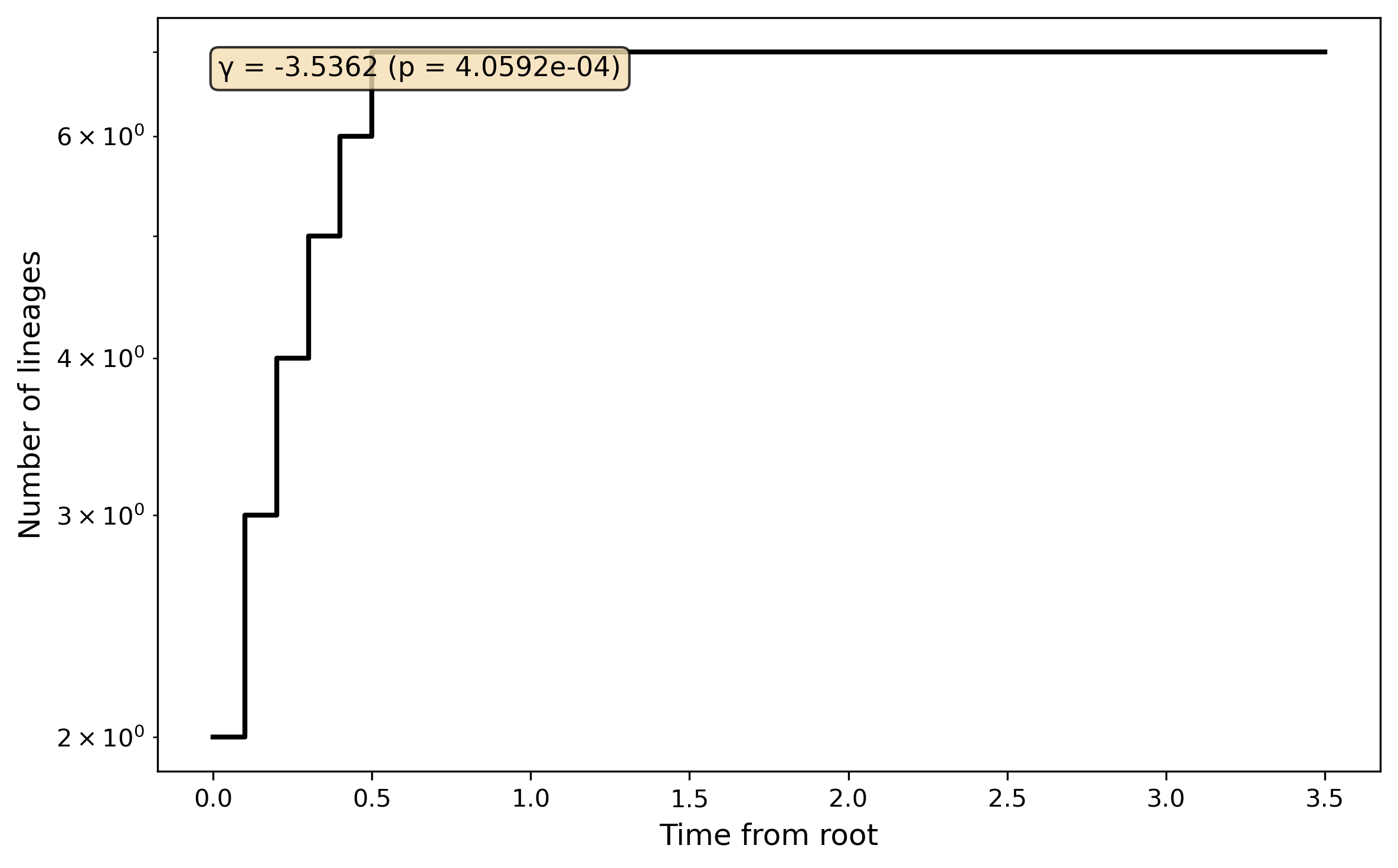
Example: recent burst (accelerating diversification)
Lineage accumulation is concentrated near the present. The significantly positive gamma (p = 0.022) indicates late diversification.
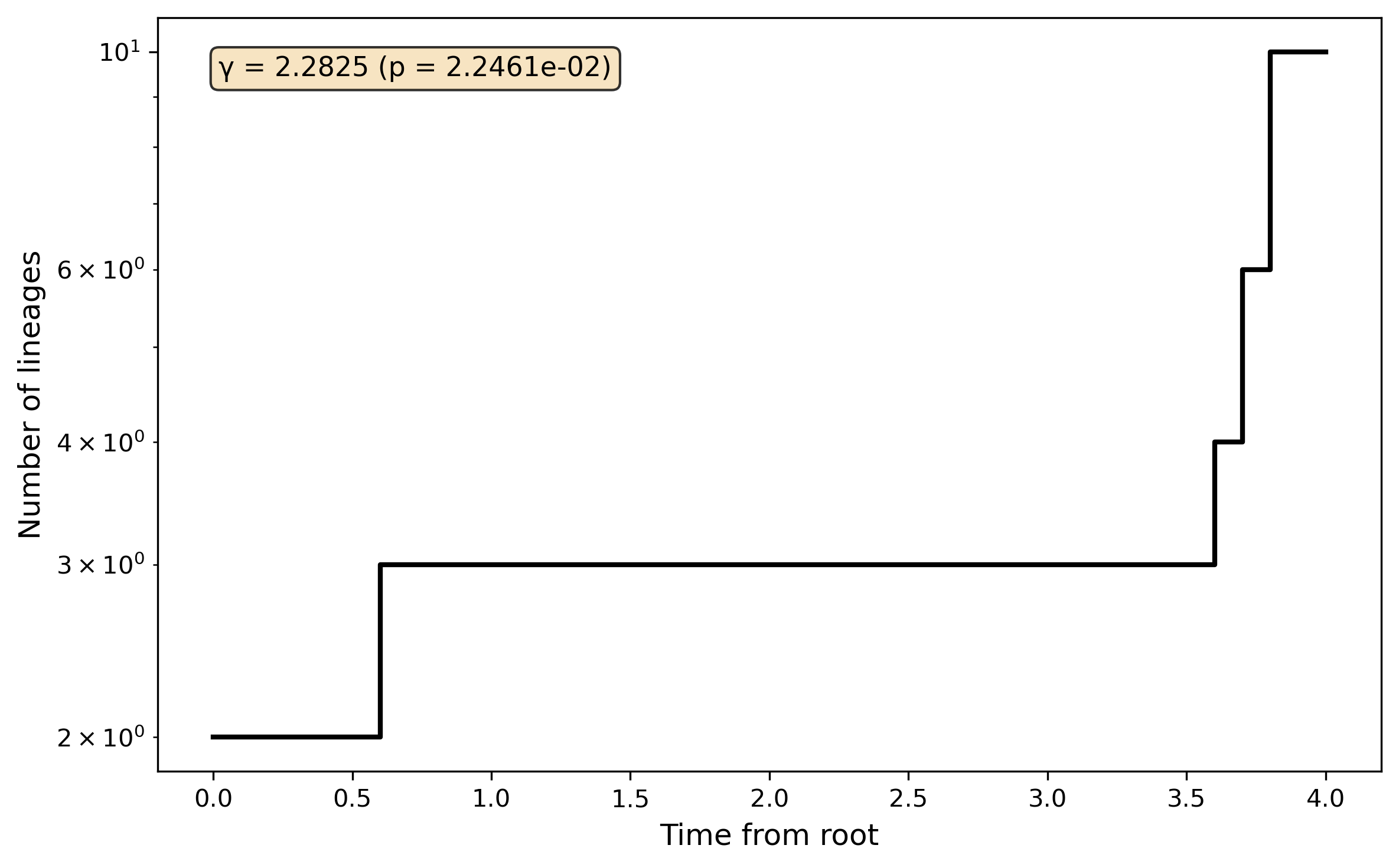
Step 3: Verbose output for downstream analysis.
phykit ltt -t gecko_dated.tre -v
Verbose mode prints branching times (node ages) and the full LTT data table (time_from_root, n_lineages), which can be piped to custom plotting or further analysis.
Validation against R's ape::gammaStat()
PhyKIT's gamma statistic was validated against R's ape package (v5.8.1, R 4.4.0). Results match to 10 decimal places:
Tree topology |
PhyKIT gamma |
R ape gamma |
|---|---|---|
Balanced 8-tip |
-1.4142135624 |
-1.4142135624 |
Ladder (caterpillar) 5-tip |
-0.7142857143 |
-0.7142857143 |
Recent burst 10-tip |
2.2824790785 |
2.2824790785 |
Early burst 7-tip |
-3.5362021857 |
-3.5362021857 |
The algorithm replicates the exact formula from ape's gammaStat.R
source, including the rev() step on internode intervals.
Long branch score
Function names: long_branch_score; lb_score; lbs
Command line interface: pk_long_branch_score; pk_lb_score; pk_lbs
Calculate long branch (LB) scores in a phylogeny.
Lower LB scores are thought to be desirable because they are indicative of taxa or trees that likely do not have issues with long branch attraction.
LB score is the mean pairwise patristic distance of taxon i compared to all other taxa divided by the average pairwise patristic distance.
PhyKIT reports summary statistics. To obtain LB scores for each taxon, use the -v/--verbose option.
LB scores are calculated following Struck, Evolutionary Bioinformatics (2014), doi: 10.4137/EBO.S14239.
phykit long_branch_score <tree> [-v/--verbose] [--json]
Options:
<tree>: first argument after function name should be a tree file
-v/--verbose: optional argument to print all LB score values
--json: optional argument to print results as JSON
Monophyly check
Function names: monophyly_check; is_monophyletic
Command line interface: pk_monophyly_check; pk_is_monophyletic
This analysis can be used to determine if a set of taxa are exclusively monophyletic. By exclusively monophyletic, if other taxa are in the same clade, the lineage will not be considered exclusively monophyletic.
Requires a taxa file, which specifies which tip names are expected to be monophyletic. File format is a single column file with tip names. Tip names not present in the tree will not be considered when examining monophyly.
The output will have six columns. col 1: if the clade was or wasn't monophyletic col 2: average bipartition support value in the clade of interest col 3: maximum bipartition support value in the clade of interest col 4: minimum bipartition support value in the clade of interest col 5: standard deviation of bipartition support values in the clade of interest col 6: tip names of taxa monophyletic with the lineage of interest excluding those that are listed in the taxa_of_interest file
phykit monophyly_check <tree> <list_of_taxa> [--json]
Options:
<tree>: first argument after function name should be a tree file
<list_of_taxa>: single column file with list of tip names to
examine the monophyly of
--json: optional argument to print results as JSON
Multi-regime OU models (OUwie)
Function names: ouwie; fit_ouwie; multi_regime_ou
Command line interface: pk_ouwie; pk_fit_ouwie; pk_multi_regime_ou
Fit multi-regime Ornstein-Uhlenbeck models of continuous trait evolution,
analogous to R's OUwie package (Beaulieu et al. 2012). Fits up to 7
models and ranks them by AICc, BIC, and AICc weights. Regime assignments
to internal branches are inferred via Fitch parsimony.
Models:
BM1 -- single-rate Brownian motion (2 params)
BMS -- multi-rate Brownian motion with per-regime sigma2 (R+1 params)
OU1 -- single-regime Ornstein-Uhlenbeck (3 params)
OUM -- multi-regime OU with per-regime trait optima (R+2 params)
OUMV -- OUM + per-regime sigma2 (2R+1 params)
OUMA -- OUM + per-regime alpha (2R+1 params)
OUMVA -- all parameters regime-specific (3R params)
Each model reports R² = 1 - (σ²_model / σ²_BM1), measuring improvement over the simplest Brownian motion baseline. For multi-regime models with per-regime σ² values, the average is used.
phykit ouwie -t <tree> -d <trait_data> -r <regime_data> [--models BM1,OUM,OUMVA] [--json]
Options:
-t/--tree: a tree file in Newick format
-d/--trait_data: tab-delimited trait file (taxon<tab>value)
-r/--regime_data: tab-delimited regime file (taxon<tab>regime_label)
--models: comma-separated list of models to fit (default: all 7)
--json: optional argument to print results as JSON
The trait data file is a two-column tab-delimited file mapping taxon names to continuous trait values:
dog  1.1
bear 1.9
raccoon      1.5
seal 1.8
sea_lion     1.8
cat  0.5
weasel       1.7
monkey       0.3
The regime data file is a two-column tab-delimited file mapping taxon names to discrete regime labels (e.g., habitat, diet category):
dog  terrestrial
bear terrestrial
raccoon      terrestrial
seal aquatic
sea_lion     aquatic
cat  terrestrial
weasel       terrestrial
monkey       terrestrial
Example output:
OUwie Model Comparison
======================
Regimes: aquatic, terrestrial

Model      logLik     AICc      BIC     k  AICc_w  Params
-----  ----------  -------  -------  ----  ------  ------
OUMVA     -6.9859  27.9717  29.5459     6  0.0040  alpha={aquatic:0.38, terrestrial:0.38}, sigma2={aquatic:0.01, terrestrial:0.05}, theta={aquatic:1.80, terrestrial:1.24}
OUMA      -6.9859  27.9717  29.0119     5  0.0040  alpha={aquatic:0.38, terrestrial:0.38}, sigma2=0.0384, theta={aquatic:1.80, terrestrial:1.24}
OUMV      -6.9859  27.9717  29.0119     5  0.0040  alpha=0.3849, sigma2={aquatic:0.01, terrestrial:0.05}, theta={aquatic:1.80, terrestrial:1.24}
OUM       -8.6297  25.2594  26.3276     4  0.0488  alpha=0.0706, sigma2=0.0329, theta={aquatic:1.80, terrestrial:1.33}
OU1      -10.2890  27.2447  28.0459     3  0.0063  alpha=0.0398, sigma2=0.0363, theta=1.64
BMS      -11.2046  29.0759  29.8771     3  0.0024  sigma2={aquatic:0.01, terrestrial:0.05}, z0=1.64
BM1      -11.5697  27.1393  27.6735     2  0.0073  sigma2=0.0384, z0=1.64

Best model (AICc): OUM
Best model (BIC): OUM
R validation: Validated against OUwie in R
(see tests/r_validation/validate_ouwie_r2.R).
Nearest neighbor interchange
Function names: nearest_neighbor_interchange; nni
Command line interface: pk_nearest_neighbor_interchange; pk_nni
Generate nearest neighbor interchange (NNI) moves for a binary rooted tree.
By default, all NNI rearrangements are emitted (one tree per neighbor),
and the output file will have the same name as the input file but with
the suffix .nnis. The input phylogeny is written at the top of the
output unless --no-input-tree is supplied.
Pass --branch (a comma-separated pair of taxa) or --branches
(a file with one pair per line) to restrict output to the two NNI
rearrangements around a specific internal branch. The branch is
identified as the edge leading to the most recent common ancestor
(MRCA) of the supplied taxa. This is useful for branch-by-branch
likelihood comparison in IQ-TREE / RAxML: re-score the bundle of
output trees against an alignment and compare site-likelihoods at the
labelled split.
phykit nearest_neighbor_interchange <tree> [-o/--output <output_file>]
    [--branch A,B] [--branches <file>] [--no-input-tree] [--json]
Options:
<tree>: first argument after function name should be a tree file
-o/--output: optional argument to specify output file name
--branch: optional argument. Two taxa separated by a comma
(e.g., --branch A,B) whose MRCA defines the internal branch to
rearrange. Emits the two alternative NNI topologies for that branch.
--branches: optional argument. Path to a file with one taxon pair per
line (comma- or tab-separated). Lines may optionally start with a label
followed by the two taxa (label<TAB>A<TAB>B), in which case the
label is echoed in the --json report. Lines that are blank or
start with # are ignored. Each pair yields two NNI trees, emitted
in the order the pairs appear.
--no-input-tree: optional argument. Omit the input phylogeny from the
top of the output file.
--json: optional argument to print summary metadata as JSON
Example: explore likelihoods around a single internal split
# Emit the input tree + the 2 NNIs around the MRCA of taxa A, B
phykit nni species.tre --branch A,B -o candidates.nwk

# Then evaluate likelihoods in IQ-TREE
iqtree -s alignment.fa -te candidates.nwk -pre nni_compare
NeighborNet
Function names: neighbor_net; nnet
Command line interface: pk_neighbor_net; pk_nnet
Construct a NeighborNet phylogenetic network from pairwise distances (Bryant & Moulton 2004). Unlike a consensus network (which summarizes conflict across gene trees), NeighborNet infers a splits graph directly from a distance matrix — analogous to Neighbor-Joining but producing a network instead of a tree.
Input is either a FASTA alignment (distances computed internally) or a pre-computed distance matrix CSV. The algorithm:
Computes pairwise distances (p-distance, identity, or Jukes-Cantor)
Builds a NJ tree to determine the circular taxon ordering
Enumerates all circular splits compatible with that ordering
Estimates split weights via non-negative least squares (NNLS)
Visualizes as a planar splits graph (Buneman graph)
# From an alignment
phykit neighbor_net -a alignment.fa -o network.pdf

# From a pre-computed distance matrix
phykit neighbor_net --distance-matrix distances.csv -o network.pdf

# With Jukes-Cantor correction
phykit neighbor_net -a alignment.fa -o network.pdf --metric jc
Options:
-a/--alignment: FASTA alignment file (computes distances internally)
--distance-matrix: pre-computed distance matrix CSV with taxon headers
-o/--output: output figure path (required)
--metric: distance metric when using -a: identity, p-distance (default), or jc (Jukes-Cantor)
--max-splits: maximum splits for visualization (default: 30)
--json: optional argument to print results as JSON
Network signal
Function names: network_signal; netsig; net_signal
Command line interface: pk_network_signal; pk_netsig; pk_net_signal
Compute phylogenetic signal (Blomberg's K and/or Pagel's lambda) on a phylogenetic network rather than a tree. This accounts for hybridization and introgression when estimating how strongly a continuous trait tracks evolutionary history.
Standard phylogenetic signal methods assume a strictly bifurcating tree.
When the true history includes reticulation, the tree-based
variance-covariance (VCV) matrix is incorrect and signal estimates
may be biased. network_signal replaces the tree VCV with a
network VCV computed using the recursive algorithm of
Bastide et al. (Systematic Biology, 2018), which properly
weights shared ancestry through both tree-like and hybrid lineages.
Polytomies (collapsed branches) in the input tree are represented as star topologies in the network VCV, which correctly models unresolved relationships as equal covariance among all children.
Two signal metrics are available (same as phylogenetic_signal):
Blomberg's K (Blomberg et al. 2003): K = 1 under Brownian motion; K < 1 = less signal than expected; K > 1 = more. P-value via permutation test. Computing K on a network is a novel capability not available in any other tool.
Pagel's lambda (Pagel 1999): lambda = 0 = no signal; lambda = 1 = full BM signal. P-value via likelihood ratio test.
Network specification — two options:
Explicit hybrid edges (
--hybrid): specify one or more reticulation events asdonor:recipient:gammawhere gamma is the inheritance probability from the donor lineage (0 < gamma < 0.5).From quartet_network JSON (
--quartet-json): auto-infer hybrid edges from the output ofphykit quartet_network --json. The command identifies taxon pairs that swap across hybrid quartets and estimates gamma from concordance factor ratios.
# With explicit hybrid edges
phykit network_signal -t <tree> -d <trait_data> --hybrid <donor:recipient:gamma> [--method both|blombergs_k|lambda] [--permutations 1000] [--json]

# With quartet_network JSON output
phykit network_signal -t <tree> -d <trait_data> --quartet-json <quartets.json> [--method both|blombergs_k|lambda] [--permutations 1000] [--json]
Options:
-t/--tree: a rooted species tree in Newick format (with branch lengths)
-d/--trait-data: tab-delimited trait file (taxon_name<tab>trait_value)
--hybrid: one or more hybrid edge specifications (donor:recipient:gamma);
donor is the source lineage, recipient receives gene flow, gamma is the
inheritance proportion from the donor (e.g., B:C:0.3)
--quartet-json: path to JSON output from phykit quartet_network --json
--method: both (default), blombergs_k, or lambda
--permutations: number of permutations for K p-value (default: 1000)
-v/--verbose: print network VCV matrix details
--json: optional argument to print results as JSON
Output for default (both) mode:
Hybrid edge: B -> C (gamma=0.3000)
Network taxa: 5
---
Blomberg's K: 0.8234 p-value: 0.0320
Pagel's lambda: 0.7651 log-likelihood: -12.3456 p-value: 0.0012
Tutorial: Wing pattern evolution in Heliconius butterflies
This example shows a realistic workflow for computing phylogenetic signal on a network, starting from gene tree discordance analysis through to signal estimation. The scenario is motivated by the Heliconius butterfly system, where H. melpomene and H. cydno are sister species that hybridize with H. heurippa, producing introgression of wing pattern genes across species boundaries (Mavárez et al., Nature, 2006).
Step 1: Identify hybridization from gene trees.
You have gene trees from 200 loci across 6 Heliconius species.
First, use quartet_network to test whether gene tree discordance
is due to ILS alone or also involves hybridization:
phykit quartet_network -t gene_trees.nwk --json > quartets.json
Examine the output to see which quartets are classified as hybrid:
# Quick summary
python -c "
import json
data = json.load(open('quartets.json'))
print(f'Tree-like: {data[\"tree_count\"]}')
print(f'Hybrid: {data[\"hybrid_count\"]}')
print(f'Unresolved: {data[\"unresolved_count\"]}')
for q in data['quartets']:
    if q['classification'] == 'hybrid':
        print(f'  {q[\"dominant_topology\"]}  CFs: {q[\"cfs\"]}')
"
Suppose the output shows that quartets involving H. melpomene and H. heurippa are consistently classified as hybrid, with asymmetric minor concordance factors — evidence of gene flow between these lineages.
Step 2a: Compute signal using quartet_network output directly.
Feed the quartet JSON into network_signal along with a rooted
species tree and wing pattern measurements (e.g., forewing red band
area, log-transformed):
phykit network_signal \
    -t species_tree.nwk \
    -d wing_pattern.tsv \
    --quartet-json quartets.json
The command automatically identifies the strongest hybrid signal from the quartet classifications and estimates the inheritance probability (gamma).
Step 2b: Alternatively, specify hybrid edges explicitly.
If you know the donor and recipient lineages (e.g., from prior knowledge or external network inference), you can specify the hybrid edge directly. Here, H. melpomene is the donor of wing pattern alleles to H. heurippa with an estimated 25% introgression:
phykit network_signal \
    -t species_tree.nwk \
    -d wing_pattern.tsv \
    --hybrid H_melpomene:H_heurippa:0.25
Step 3: Interpret the results.
Example output:
Hybrid edge: H_melpomene -> H_heurippa (gamma=0.2500)
Network taxa: 6
---
Blomberg's K: 0.6821    p-value: 0.0410
Pagel's lambda: 0.5934    log-likelihood: -8.7231    p-value: 0.0085
Interpretation:
K = 0.68 (p = 0.04): significant phylogenetic signal, but less than expected under Brownian motion (K < 1). This is consistent with the wing pattern being phylogenetically conserved in most lineages but displaced in H. heurippa due to introgression from H. melpomene.
Lambda = 0.59 (p = 0.009): moderate phylogenetic signal. The trait is not evolving independently of the network (lambda > 0), but the fit is better with reduced covariance (lambda < 1).
Comparison with tree-based signal: running
phylogenetic_signalon the species tree alone would likely produce a lower K value because the tree VCV does not account for the shared ancestry introduced by introgression. The network-based K is a more accurate estimate of how much evolutionary history explains trait variation.
Why this matters: Without accounting for the network, the tree treats H. heurippa's wing pattern as an independent observation. In reality, its wing pattern was partly inherited from H. melpomene through hybridization — the network VCV correctly reflects this shared ancestry, producing a more accurate phylogenetic signal estimate.
Algorithm — Bastide et al. 2018 network VCV
For Brownian motion on a network, the trait at a hybrid node h with parents p1 and p2 is:
X_h = gamma * (X_p1 + noise_1) + (1-gamma) * (X_p2 + noise_2)
The network VCV is computed recursively in topological order:
Tree node c with parent p, edge length l:
V[c,c] = V[p,p] + l
V[c,j] = V[p,j]for all other nodes jHybrid node h with parents p1 (weight gamma) and p2 (weight 1-gamma):
V[h,h] = gamma^2 * (V[p1,p1] + l1) + (1-gamma)^2 * (V[p2,p2] + l2) + 2*gamma*(1-gamma)*V[p1,p2]
V[h,j] = gamma * V[p1,j] + (1-gamma) * V[p2,j]
The tip-by-tip submatrix is the VCV used for K and lambda.
OU shift detection (l1ou)
Function names: ou_shift_detection; ou_shifts; l1ou; detect_shifts
Command line interface: pk_ou_shift_detection; pk_ou_shifts; pk_l1ou; pk_detect_shifts
Automatic OU shift detection using the LASSO-based approach from Khabbazian et al. (2016). Discovers where on the phylogeny the adaptive optimum changed without requiring an a priori regime assignment. Only a tree and continuous trait data are needed.
The algorithm:
Fits a single-regime OU model to estimate alpha (selection strength)
Builds a design matrix with one column per candidate shift edge
Uses Cholesky transformation to remove phylogenetic correlation
Runs a LASSO path to identify candidate shift configurations
Selects the best model using pBIC, BIC, or AICc
phykit l1ou -t <tree> -d <trait_data> [--criterion pBIC] [--max-shifts N] [--json]
Options:
-t/--tree: a tree file in Newick format
-d/--trait_data: tab-delimited trait file (taxon<tab>value)
--criterion: model selection criterion: pBIC (default), BIC, or AICc
--max-shifts: maximum number of shifts to consider (default: n/2)
--json: optional argument to print results as JSON
Example output (no shifts detected):
============================================================
OU Shift Detection (l1ou)
============================================================
Number of tips:       8
Number of shifts:     0
Selection criterion:  pBIC
Alpha (OU strength):  0.784803
Sigma² (BM rate):     1.203455
Root optimum (θ₀):    1.206251
Log-likelihood:       -10.2890
pBIC:                 26.8163
BIC:                  26.8163
AICc:                 32.5780

No shifts detected — single-regime OU is best.
============================================================
Example output (shifts detected):
============================================================
OU Shift Detection (l1ou)
============================================================
Number of tips:       100
Number of shifts:     8
Selection criterion:  pBIC
Alpha (OU strength):  0.606894
Sigma² (BM rate):     0.062519
Root optimum (θ₀):    0.248810
Log-likelihood:       48.6896
pBIC:                 17.6266
BIC:                  -9.8811
AICc:                 -49.8793

Detected shifts:
------------------------------------------------------------
  Shift 1: terminal branch to valencienni
           New optimum: -0.564678
  Shift 2: terminal branch to insolitus
           New optimum: -0.876398
  Shift 3: stem of (barbatus, porcus, ... +2 more)
           New optimum: -0.635087
  Shift 4: stem of (altitudinalis, oporinus, ... +13 more)
           New optimum: -0.462944
============================================================
Results have been validated against R's l1ou package (Khabbazian et al. 2016). On a 100-tip lizard dataset, PhyKIT recovers the same 8 adaptive shifts with matching alpha (0.607) and pBIC (17.6 vs R's 16.8).
Parsimony score
Function names: parsimony_score; parsimony; pars
Command line interface: pk_parsimony_score; pk_parsimony; pk_pars
Compute the Fitch (1971) maximum parsimony score of a tree given an alignment. The parsimony score is the minimum number of character state changes required to explain the alignment on the given tree topology. Gap characters (-, N, X, ?) are treated as wildcards.
Cross-validated against R's phangorn::parsimony(method="fitch").
phykit parsimony_score -t <tree> -a <alignment> [-v/--verbose] [--json]
Options:
-t/--tree: tree file (required)
-a/--alignment: alignment file in FASTA format (required)
-v/--verbose: print per-site parsimony scores
--json: optional argument to print results as JSON
R validation: Validated against phangorn in R
(see tests/r_validation/validate_parsimony.R).
Patristic distances
Function names: patristic_distances; pd
Command line interface: pk_patristic_distances; pk_pd
Calculate summary statistics among patristic distances in a phylogeny.
Patristic distances are all tip-to-tip distances in a phylogeny.
To obtain all patristic distances, use the -v/--verbose option. With the -v option, the first column will have two taxon names separated by a '-' followed by the patristic distance. Features will be tab separated.
phykit patristic_distances <tree> [-v/--verbose] [--json]
Options:
<tree>: first argument after function name should be a tree file
-v/--verbose: optional argument to print all tip-to-tip distances
--json: optional argument to print results as JSON
Phenogram (traitgram)
Function names: phenogram; traitgram; tg
Command line interface: pk_phenogram; pk_traitgram; pk_tg
Plot a phenogram (traitgram) showing trait evolution along a phylogeny
(analogous to R's phytools::phenogram()). The X-axis represents
distance from the root and the Y-axis represents trait values.
Ancestral states are reconstructed via maximum-likelihood.
phykit phenogram -t <tree> -d <trait_data> -o <output.png>
    [--fig-width <float>] [--fig-height <float>] [--dpi <int>] [--no-title] [--title <str>]
    [--legend-position <str>] [--ylabel-fontsize <float>] [--xlabel-fontsize <float>]
    [--title-fontsize <float>] [--axis-fontsize <float>] [--colors <str>] [--ladderize] [--cladogram] [--circular] [--color-file <file>] [--json]
Options:
-t/--tree: a tree file in Newick format
-d/--trait_data: tab-delimited trait file (taxon<tab>value)
-o/--output: output plot file path (required)
--fig-width: figure width in inches (auto-scaled if omitted)
--fig-height: figure height in inches (auto-scaled if omitted)
--dpi: resolution in DPI (default: 300)
--no-title: hide the plot title
--title: custom title text
--legend-position: legend location (e.g., "upper right", "none" to hide)
--ylabel-fontsize: font size for y-axis labels; 0 to hide
--xlabel-fontsize: font size for x-axis labels; 0 to hide
--title-fontsize: font size for the title
--axis-fontsize: font size for axis labels
--colors: comma-separated colors (hex or named)
--ladderize: ladderize (sort) the tree before plotting
--cladogram: draw cladogram (equal branch lengths, tips aligned) instead of phylogram
--circular: draw circular (radial/fan) phylogram instead of rectangular
--color-file: color annotation file for tip labels, clade ranges, and branch colors (iTOL-inspired TSV format)
--json: optional argument to print results as JSON
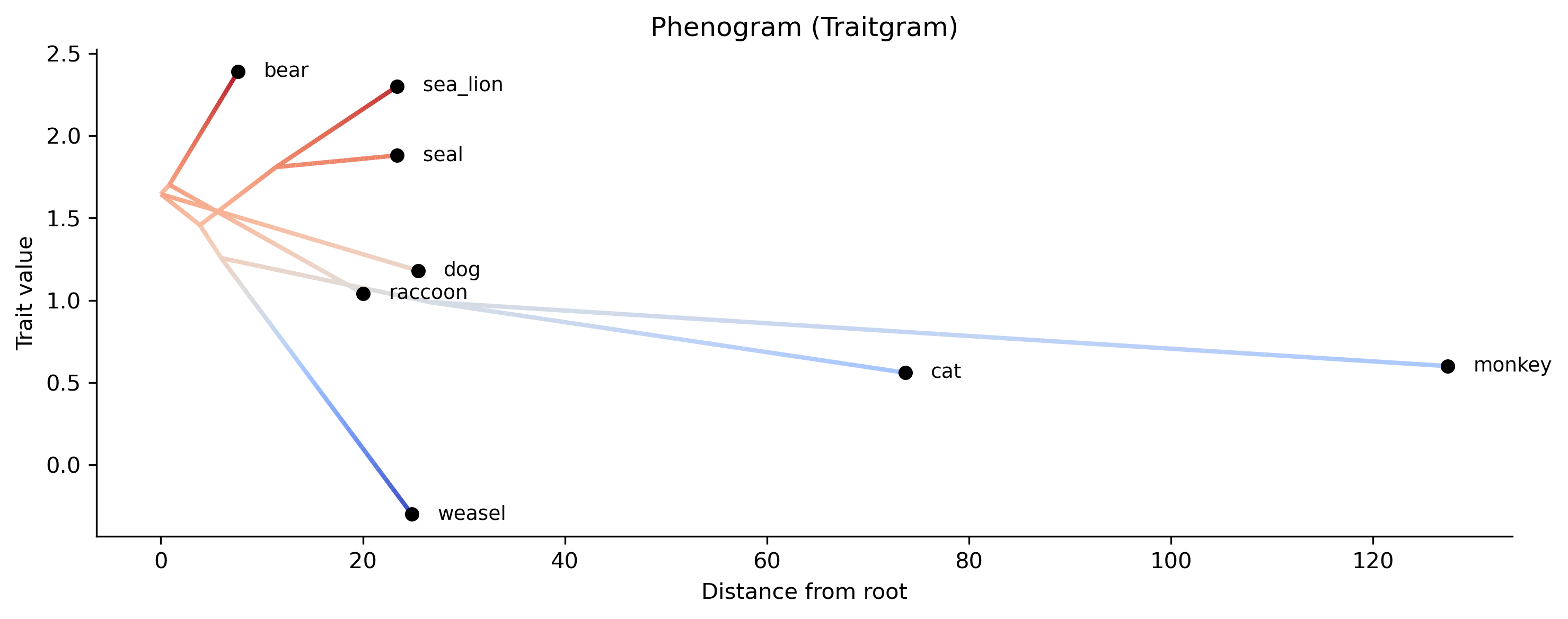
Phylogenetic ANOVA / MANOVA
Function names: phylo_anova; panova; phylo_manova; pmanova
Command line interface: pk_phylo_anova; pk_panova; pk_phylo_manova; pk_pmanova
Phylogenetic ANOVA (univariate) or MANOVA (multivariate) using the Residual Randomization Permutation Procedure (RRPP) of Adams & Collyer (2018). Tests whether a continuous trait or multiple traits differ across discrete groups (e.g., diet, habitat) while accounting for phylogenetic non-independence via the phylogenetic variance-covariance matrix.
The method auto-detects univariate vs multivariate based on the number
of response trait columns. With one response trait, it runs a phylogenetic
ANOVA; with multiple, it runs a phylogenetic MANOVA using Pillai's trace
as the test statistic. Users can override with --method anova or
--method manova.
How it works:
The phylogenetic VCV matrix is Cholesky-decomposed and used to transform the data, removing phylogenetic correlation.
A reduced model (intercept only) and full model (intercept + group) are fit to the transformed data.
The observed F-statistic (ANOVA) or Pillai's trace (MANOVA) is computed.
Residuals of the reduced model are permuted (RRPP) to build a null distribution; the p-value is the proportion of permuted statistics >= the observed statistic.
A Z-score (effect size) is also reported.
Interpreting the output:
The ANOVA table shows:
SS (Sum of Squares): variance attributed to the grouping factor vs residuals.
MS (Mean Squares): SS / Df.
F: ratio of MS_model to MS_residual. Larger F means greater group separation relative to within-group variation.
Z: standardized effect size — how many standard deviations the observed F is from the null mean. Z > 2 generally indicates strong signal.
p-value: proportion of permuted F values >= observed. Small p (e.g., < 0.05) suggests groups differ significantly after accounting for phylogeny.
Pillai's trace (MANOVA only): ranges from 0 to the number of response traits. Higher values indicate stronger multivariate group separation.
A non-significant result (large p-value) means that after accounting for shared ancestry, the groups do not differ more than expected by chance. This is common when closely related species share similar trait values regardless of group assignment.
Pairwise comparisons (--pairwise): for each pair of groups,
computes the Euclidean distance between group means in phylogenetically
transformed space, with permutation-based p-values.
Example (ANOVA):
phykit phylo_anova -t species.tre --traits trait_data.tsv --permutations 999
Example output:
Phylogenetic ANOVA (RRPP, 999 permutations)
Response: body_mass
Groups (3): carnivore, herbivore, omnivore
N taxa: 8

Source             Df           SS           MS          F          Z    p-value
----------------------------------------------------------------------------
group               2       0.0382       0.0191     0.3548    -0.7213     0.8088
residuals           5       0.2691       0.0538
total               7       0.3073
In this example, p = 0.81 and Z = -0.72 indicate no significant difference in body mass among diet groups after accounting for phylogeny.
Example (MANOVA with pairwise):
phykit phylo_manova -t species.tre --traits multi_traits.tsv --pairwise --permutations 999
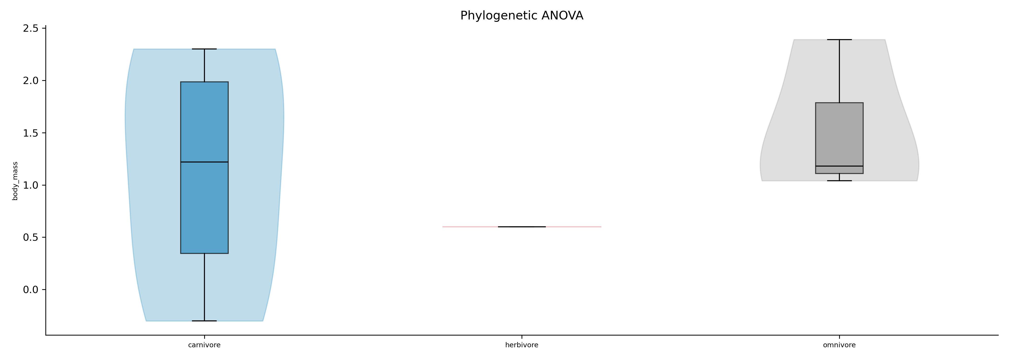
Violin + boxplot showing trait values by group for phylogenetic ANOVA.
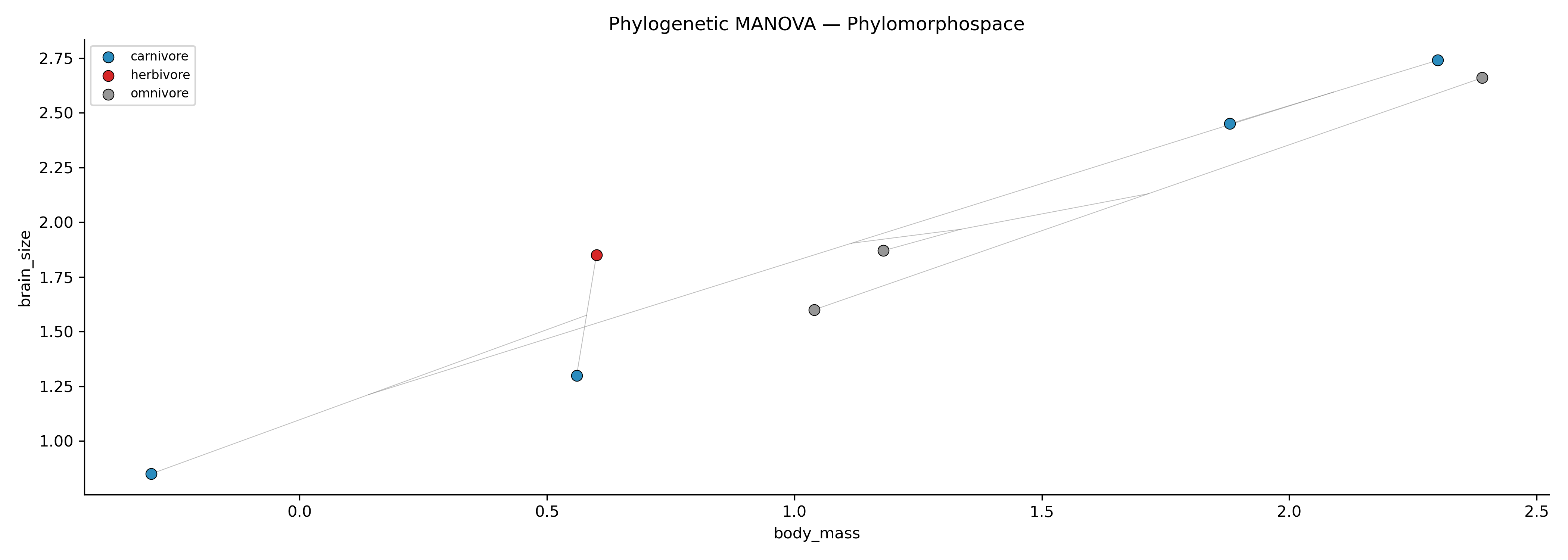
Phylomorphospace colored by group for phylogenetic MANOVA. Points represent species, edges represent phylogenetic relationships, and colors correspond to group membership.
phykit phylo_anova -t <tree> --traits <traits_file>
    [--group-column <name>] [--method auto|anova|manova]
    [--permutations <int>] [--pairwise]
    [--plot-output <file>] [--plot-type boxplot|phylomorphospace]
    [--seed <int>] [--json]
Options:
-t/--tree: species tree file (required)
--traits: TSV file with taxon, group column, and one or more response trait columns (required)
--group-column: name of the categorical grouping column (default: first non-taxon column)
--method: auto, anova, or manova (default: auto — detects from number of response columns)
--permutations: number of RRPP permutations (default: 1000)
--pairwise: include post-hoc pairwise group comparisons
--plot-output: output figure path (.png, .pdf, .svg)
--plot-type: boxplot (violin+boxplot for ANOVA) or phylomorphospace (for MANOVA); default: auto-detected
--seed: random seed for reproducible permutations
--json: output results as JSON
R validation: Deterministic components (SS, MS, F, Pillai's trace)
have been validated against manual Cholesky-transformed ANOVA/MANOVA
in R using ape::vcv() for the phylogenetic covariance matrix
(see tests/r_validation/validate_phylo_anova.R).
Phylogenetic GLM
Function names: phylogenetic_glm; phylo_glm; pglm
Command line interface: pk_phylogenetic_glm; pk_phylo_glm; pk_pglm
Fit a Phylogenetic Generalized Linear Model (GLM) for binary or count response data while accounting for phylogenetic non-independence among species.
Two families are supported:
binomial: logistic regression via Maximum Penalized Likelihood Estimation (logistic_MPLE; Ives & Garland 2010). Uses Firth's penalty to prevent bias from complete/quasi-complete separation, and jointly estimates the phylogenetic signal parameter alpha via a two-state continuous-time Markov chain on the tree.
poisson: Poisson regression via Generalized Estimating Equations (poisson_GEE; Paradis & Claude 2002). Uses Fisher scoring with the phylogenetic correlation matrix and reports an overdispersion parameter.
The multi-trait input file should be tab-delimited with a header row:
taxon<tab>trait1<tab>trait2<tab>...
Output includes coefficient estimates, standard errors, z-values, p-values, log-likelihood, AIC, and McFadden's pseudo-R² (computed from full vs. intercept-only model log-likelihoods).
phykit phylogenetic_glm -t <tree> -d <trait_data> -y <response> -x <predictor1> [predictor2 ...] --family <binomial|poisson> [-g <gene_trees>] [--json]
Options:
-t/--tree: a tree file in Newick format
-d/--trait_data: tab-delimited multi-trait file with header row
-y/--response: response (dependent) variable column name
-x/--predictors: one or more predictor column names
--family: distribution family: binomial or poisson
--method: estimation method: logistic_MPLE or poisson_GEE (auto from family)
--btol: linear predictor bound for logistic model (default: 10)
--log-alpha-bound: bound on log(alpha) for logistic model (default: 4)
-g/--gene-trees: optional multi-Newick file of gene trees; when provided, uses a discordance-aware VCV (genome-wide average) instead of the species-tree VCV
--json: optional argument to print results as JSON
R validation: Validated against phylolm in R
(see tests/r_validation/validate_glm_pseudo_r2.R).
Phylogenetic heatmap
Function names: phylo_heatmap; pheatmap; ph
Command line interface: pk_phylo_heatmap; pk_pheatmap; pk_ph
Draw a phylogenetic heatmap: a phylogeny alongside a color-coded matrix of numeric trait values, with rows aligned to tree tips. Analogous to R's phytools::phylo.heatmap().
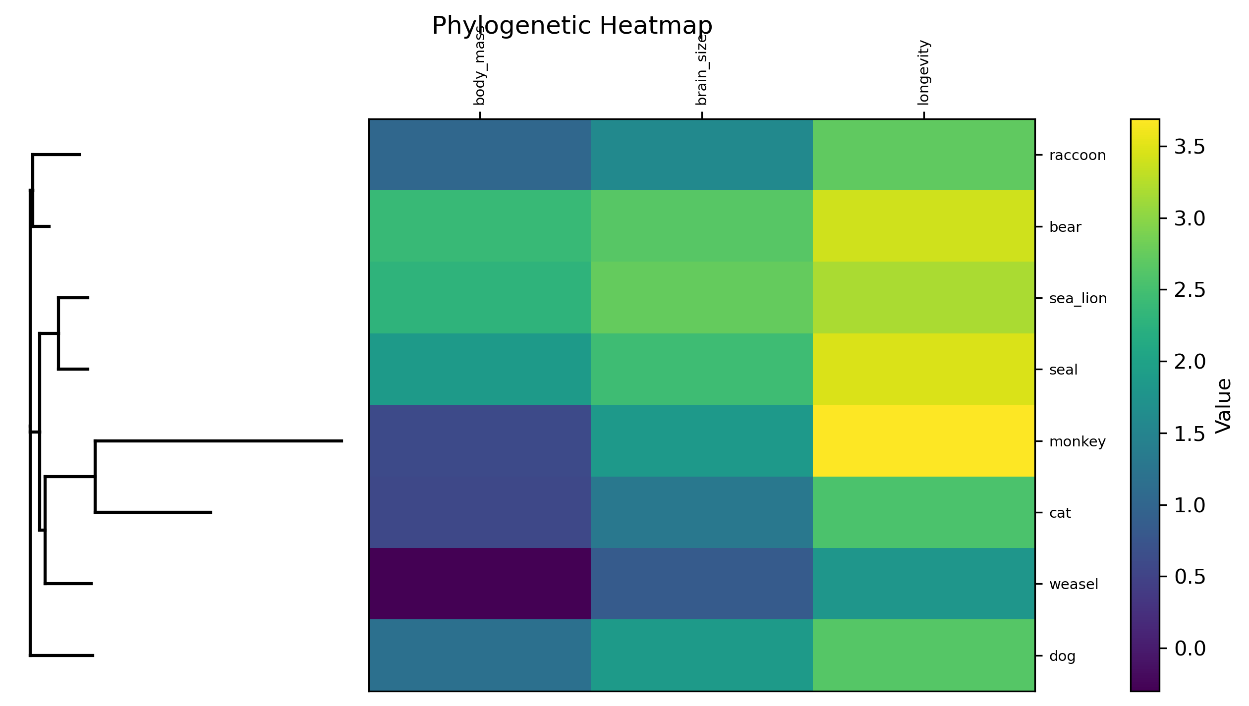
phykit phylo_heatmap -t <tree> -d <data> -o <output>
        [--split 0.3] [--standardize] [--cmap viridis] [--cluster-columns] [--json]
Options:
-t/--tree: tree file (required)
-d/--data: numeric data matrix in TSV format with header row (required)
-o/--output: output figure path (required; supports .png, .pdf, .svg)
--split: fraction of figure width for the tree panel (default: 0.3)
--standardize: z-score each column before coloring
--cmap: matplotlib colormap name (default: viridis)
--cluster-columns: cluster trait columns by similarity and display a dendrogram at the top
--json: optional argument to output metadata as JSON
Phylogenetic imputation
Function names: phylo_impute; impute; phylo_imp
Command line interface: pk_phylo_impute; pk_impute; pk_phylo_imp
Impute missing continuous trait values using phylogenetic relationships
and between-trait correlations under Brownian motion. Missing values
(NA, ?, or empty) in a multi-trait TSV are predicted from:
Phylogenetic neighbors: closely related species with observed values contribute more to the imputation via the phylogenetic VCV
Trait correlations: if a taxon has observed values for other traits, between-trait covariance improves the prediction
Reports imputed values with standard errors and 95% confidence intervals. The output TSV is a drop-in replacement for the input with all missing values filled in.
phykit phylo_impute -t <tree> -d <trait_data> -o <output> [--json]
phykit phylo_impute -t <tree> -d <trait_data> -o <output> -g <gene_trees>
Options:
-t/--tree: tree file in Newick format (required)
-d/--trait-data: multi-trait TSV with header; missing values as NA, ?, or empty (required)
-o/--output: output TSV file with imputed values (required)
-g/--gene-trees: gene trees for discordance-aware VCV
--json: optional argument to print results as JSON
R validation: Validated against Rphylopars in R
(see tests/r_validation/validate_phylo_impute.R).
Phylogenetic Logistic Regression
Function names: phylo_logistic; phylo_logreg; plogreg
Command line interface: pk_phylo_logistic; pk_phylo_logreg; pk_plogreg
Fit a Phylogenetic Logistic Regression for binary (0/1) response data while accounting for phylogenetic non-independence among species (Ives & Garland 2010).
Uses Maximum Penalized Likelihood Estimation (logistic_MPLE) with Firth's bias-correction penalty and jointly estimates the phylogenetic signal parameter alpha via the OU-transformed variance-covariance matrix.
The multi-trait input file should be tab-delimited with a header row:
taxon<tab>trait1<tab>trait2<tab>...
Output includes coefficient estimates, standard errors, z-values, p-values, alpha, log-likelihood, penalized log-likelihood, and AIC.
phykit phylo_logistic -t <tree> -d <trait_data> --response <column> --predictor <column> [--method logistic_MPLE|logistic_IG10] [--json]
Options:
-t/--tree: a tree file in Newick format
-d/--trait-data: tab-delimited multi-trait file with header row
--response: binary response column name (must contain only 0 and 1)
--predictor: predictor column name(s), comma-separated for multiple
--method: estimation method: logistic_MPLE or logistic_IG10 (default: logistic_MPLE)
--json: optional argument to print results as JSON
R validation: Validated against phylolm in R
(see tests/r_validation/validate_phylo_logistic.R).
Phylogenetic Ordination
Function names: phylogenetic_ordination; phylo_ordination; ordination; ord;
phylo_pca; phyl_pca; ppca; phylo_dimreduce; dimreduce; pdr
Command line interface: pk_phylogenetic_ordination; pk_phylo_ordination;
pk_ordination; pk_ord; pk_phylo_pca; pk_phyl_pca; pk_ppca;
pk_phylo_dimreduce; pk_dimreduce; pk_pdr
Perform phylogenetic ordination (PCA, t-SNE, or UMAP) on continuous multi-trait data while accounting for phylogenetic non-independence among species.
All methods use GLS-centering via the phylogenetic variance-covariance matrix. For PCA, eigendecomposition of the evolutionary rate matrix is performed to extract principal components. For t-SNE and UMAP, nonlinear embedding is applied to the GLS-centered data.
Three ordination methods are available via --method:
pca (default): phylogenetic PCA (Revell 2009). Performs eigendecomposition of the evolutionary rate matrix.
tsne: t-SNE embedding of the GLS-centered data. Perplexity is auto-set to
min(30, (n-1)/3); requires at least 4 taxa.umap: UMAP embedding of the GLS-centered data. n_neighbors is auto-set to
min(15, n-1); requires at least 3 taxa.
Two phylogenetic correction modes are available via --correction:
BM (default): assumes traits evolved under Brownian motion. The phylogenetic VCV matrix is used directly.
lambda: jointly estimates a single Pagel's lambda parameter across all traits by maximum likelihood, then rescales the off-diagonal elements of the VCV matrix. This accounts for deviations from Brownian motion.
For PCA, two modes are available via --mode:
cov (default): PCA on the evolutionary rate (covariance) matrix.
corr: PCA on the evolutionary rate correlation matrix, which standardizes traits to equal variance before extracting components.
The multi-trait input file should be tab-delimited with a header row:
taxon<tab>trait1<tab>trait2<tab>...
Lines starting with '#' are treated as comments. If the tree and trait file
have different taxa, the intersection is used and warnings are printed to
stderr.
PCA output includes eigenvalues with proportion of variance explained, trait
loadings, and taxon scores for each principal component. t-SNE/UMAP output
includes method parameters and embedding coordinates. When correction=lambda
is used, the estimated lambda and log-likelihood are also reported.
PCA results have been benchmarked against the R package
phytools
(phyl.pca function; Revell 2012). Eigenvalues, loadings, and scores match
phytools across all method/mode combinations (BM+cov, BM+corr, lambda+cov,
lambda+corr) within numerical tolerance (1e-4).
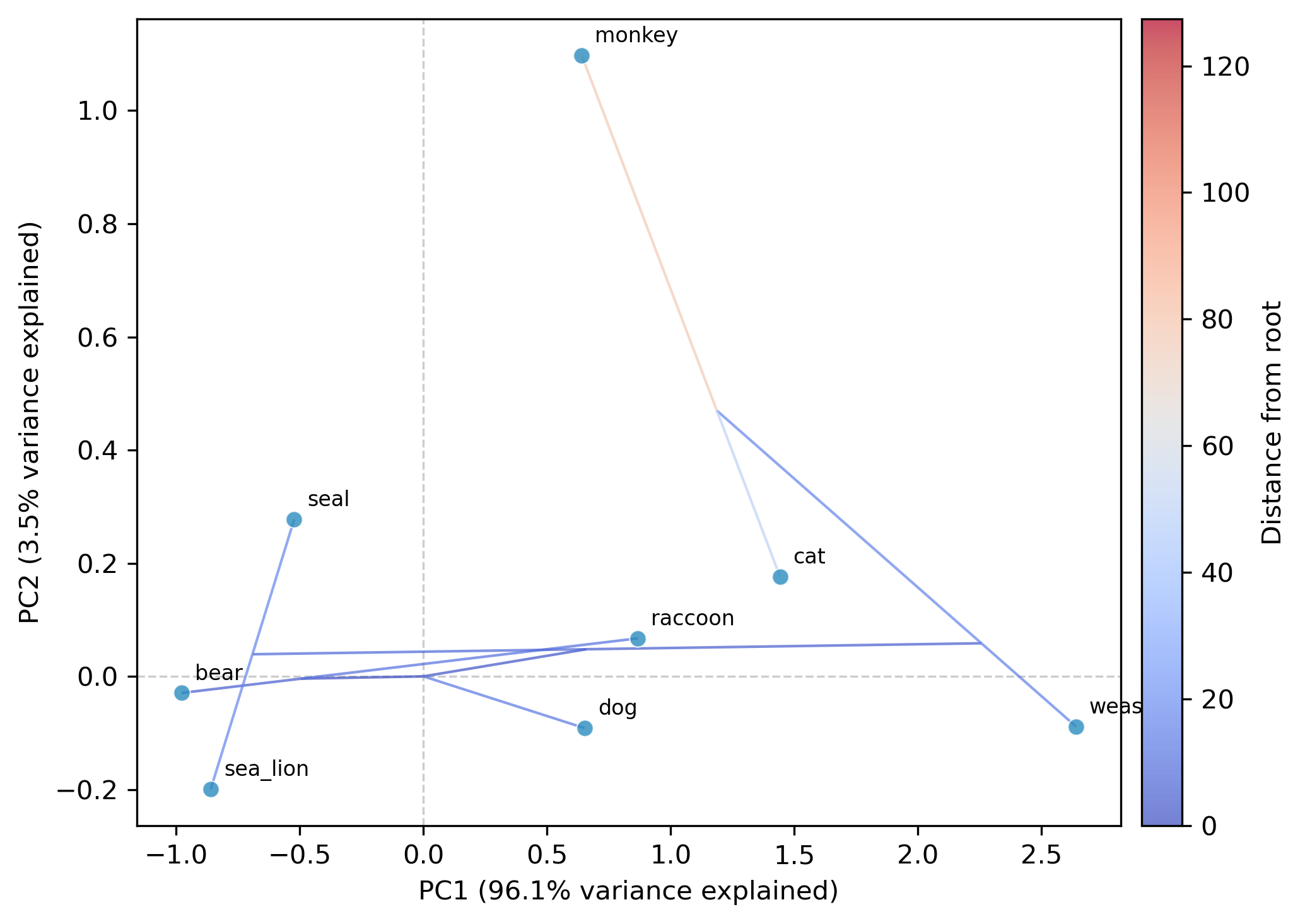
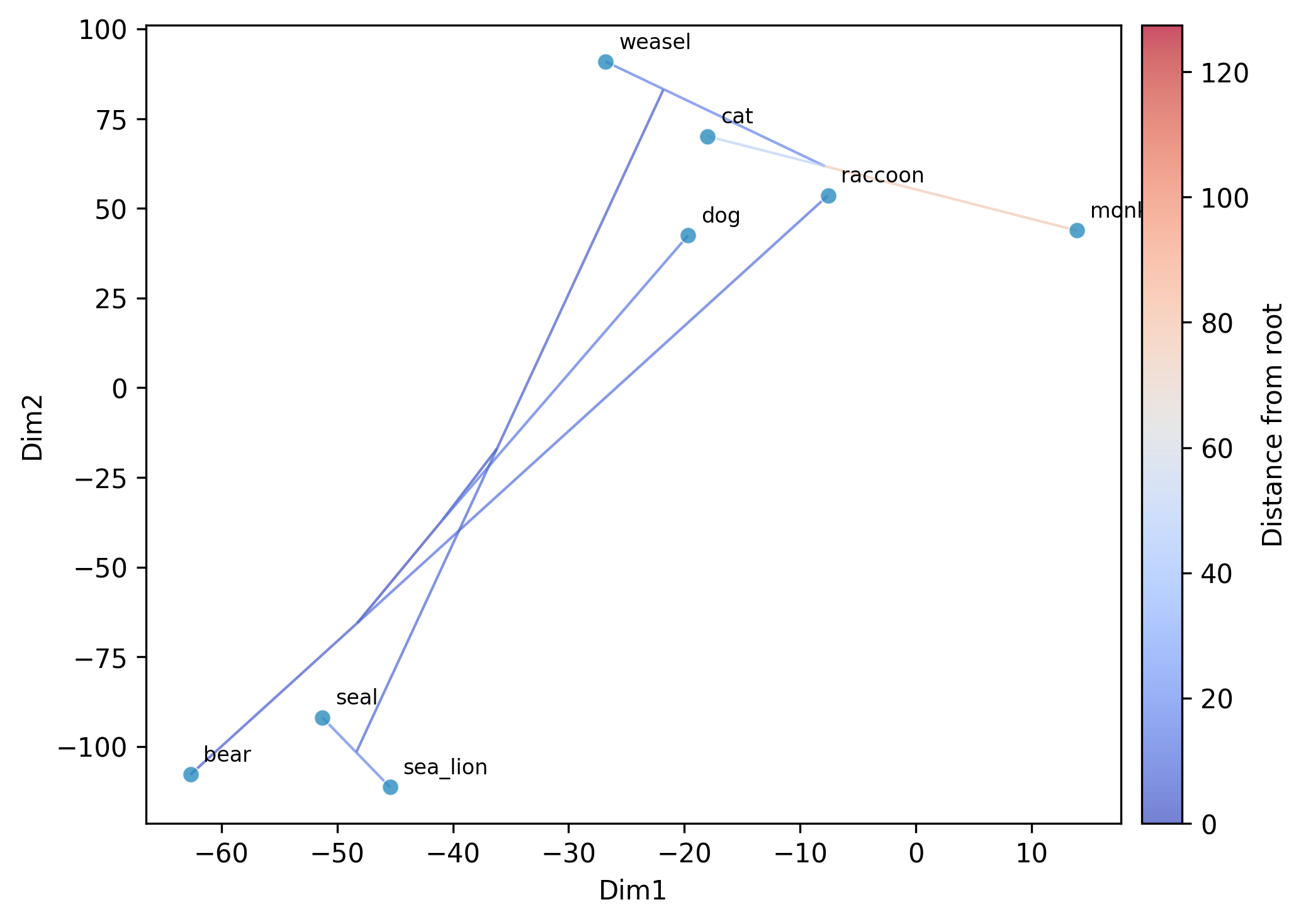
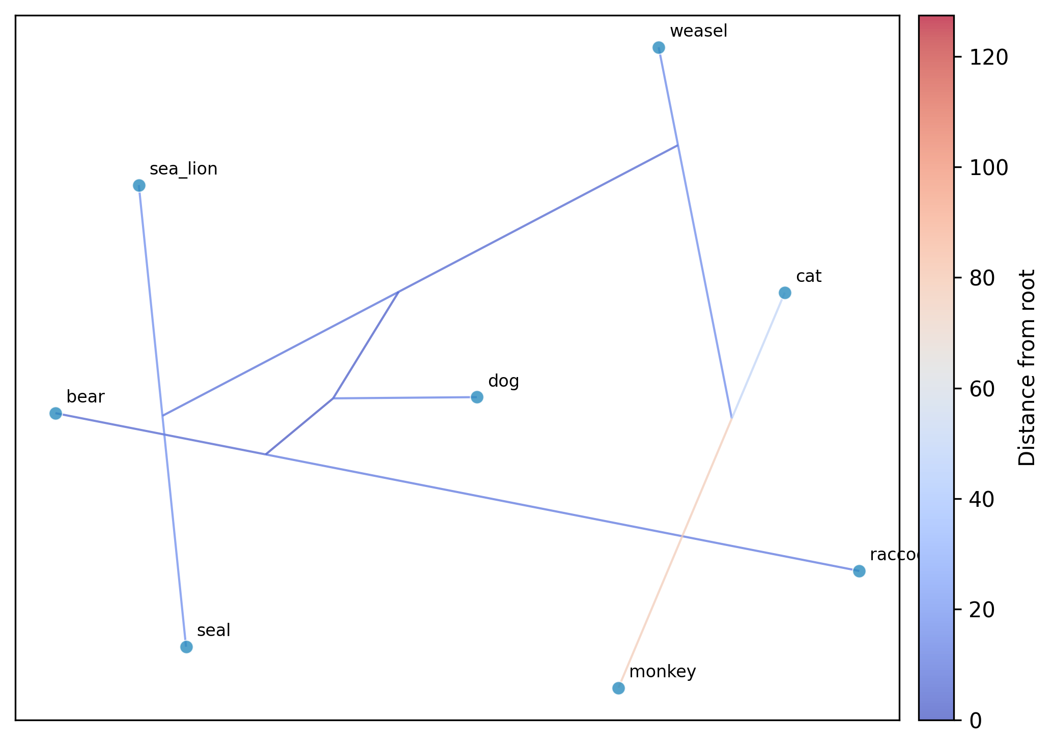
phykit phylogenetic_ordination -t <tree> -d <trait_data> [--method <pca|tsne|umap>] [--correction <BM|lambda>] [--mode <cov|corr>] [--n-components <int>] [--perplexity <float>] [--n-neighbors <int>] [--min-dist <float>] [--seed <int>] [--plot] [--plot-tree] [--no-plot-tree] [--color-by <col_or_file>] [--tree-color-by <col_or_file>] [--plot-output <path>] [-g <gene_trees>]
    [--fig-width <float>] [--fig-height <float>] [--dpi <int>] [--no-title] [--title <str>]
    [--legend-position <str>] [--ylabel-fontsize <float>] [--xlabel-fontsize <float>]
    [--title-fontsize <float>] [--axis-fontsize <float>] [--colors <str>] [--ladderize] [--cladogram] [--circular] [--color-file <file>] [--json]
Options:
-t/--tree: a tree file in Newick format
-d/--trait_data: tab-delimited multi-trait file with header row
--method: ordination method: pca, tsne, or umap (default: pca)
--correction: phylogenetic correction: BM or lambda (default: BM)
--mode: PCA mode: cov or corr (default: cov; PCA only)
--n-components: number of embedding dimensions (default: 2; tsne/umap only)
--perplexity: t-SNE perplexity (default: auto)
--n-neighbors: UMAP n_neighbors (default: auto)
--min-dist: UMAP min_dist (default: 0.1)
--seed: random seed for reproducibility
--plot: optional argument to save a scatter plot
--plot-tree: overlay the phylogeny via ancestral reconstruction (default for tsne/umap; opt-in for pca)
--no-plot-tree: disable the phylogeny overlay for tsne/umap plots
--color-by: color tip points by a trait; specify a column name from the multi-trait file or a separate tab-delimited file (taxon<tab>value) for continuous or discrete coloring
--tree-color-by: color phylogeny edges by a trait; specify a column name or a tab-delimited file (default: distance from root)
--plot-output: output path for plot (default: phylo_ordination_plot.png)
-g/--gene-trees: optional multi-Newick file of gene trees; when provided, uses a discordance-aware VCV (genome-wide average) instead of the species-tree VCV
--fig-width: figure width in inches (auto-scaled if omitted)
--fig-height: figure height in inches (auto-scaled if omitted)
--dpi: resolution in DPI (default: 300)
--no-title: hide the plot title
--title: custom title text
--legend-position: legend location (e.g., "upper right", "none" to hide)
--ylabel-fontsize: font size for y-axis labels; 0 to hide
--xlabel-fontsize: font size for x-axis labels; 0 to hide
--title-fontsize: font size for the title
--axis-fontsize: font size for axis labels
--colors: comma-separated colors (hex or named)
--ladderize: ladderize (sort) the tree before plotting
--cladogram: draw cladogram (equal branch lengths, tips aligned) instead of phylogram
--circular: draw circular (radial/fan) phylogram instead of rectangular
--color-file: color annotation file for tip labels, clade ranges, and branch colors (iTOL-inspired TSV format)
--json: optional argument to print results as JSON
Phylogenetic path analysis
Function names: phylo_path; ppath; phylopath
Command line interface: pk_phylo_path; pk_ppath; pk_phylopath
Phylogenetic path analysis (von Hardenberg & Gonzalez-Voyer 2013). Compare competing causal hypotheses (DAGs) about trait evolution while accounting for phylogenetic non-independence, using Shipley's d-separation test combined with PGLS.
How it works:
Define a set of candidate causal models as directed acyclic graphs (DAGs). Each DAG specifies which traits causally influence which other traits.
For each DAG, derive the basis set — the minimal set of conditional independence claims implied by the graph (Shipley 2000).
Test each independence claim using PGLS with Pagel's lambda. If the predictor is non-significant after conditioning, the independence holds.
Combine p-values into Fisher's C statistic. A model with a high p-value (C-test) is consistent with the data; a low p-value means the model is rejected.
Rank models by CICc (C-statistic Information Criterion, corrected for sample size). Lower CICc = better fit.
Estimate path coefficients (standardized PGLS regression slopes) and conditionally average them across well-supported models weighted by CICc.
Interpreting the output:
CICc and weights: models with delta CICc < 2 have substantial support. Weights sum to 1 and represent relative evidence.
Model p-value: p > 0.05 means the data are consistent with the DAG's independence claims. A rejected model (p < 0.05) has causal structure contradicted by the data.
Path coefficients: standardized (z-scored) regression slopes. Positive = positive causal effect; magnitude indicates strength. CIs not overlapping zero indicate significance.
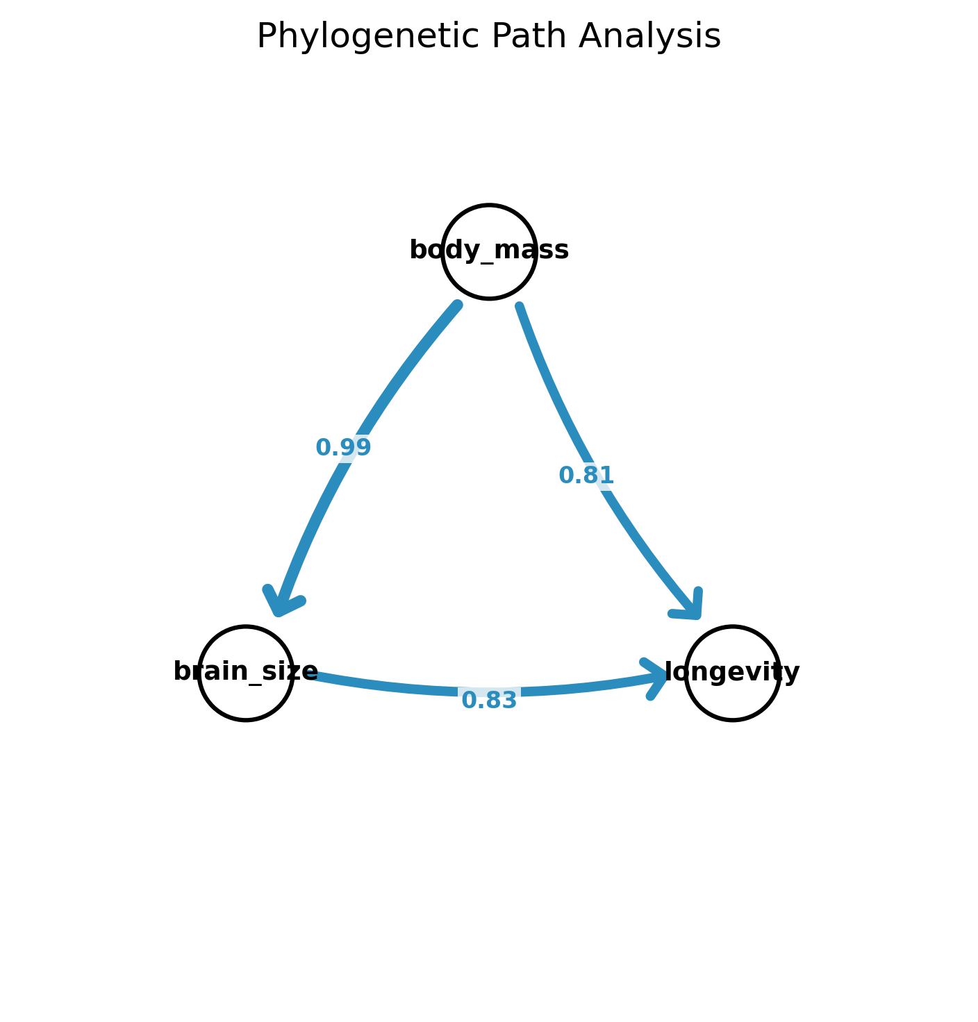
DAG plot showing model-averaged path coefficients. Blue = positive effect, line thickness proportional to coefficient magnitude.
Model file format:
# model_name: edge1, edge2, ...
direct: body_mass->brain_size, body_mass->longevity
mediated: body_mass->brain_size, brain_size->longevity
full: body_mass->brain_size, body_mass->longevity, brain_size->longevity
phykit phylo_path -t <tree> --traits <traits_file> --models <models_file>
    [--best-only] [--plot-output <file>] [--csv <file>] [--json]
Options:
-t/--tree: species tree file (required)
--traits: TSV file with taxon and continuous trait columns (required)
--models: model definition file with candidate DAGs (required)
--best-only: report only best model coefficients instead of model averaging
--plot-output: output DAG plot file (.png, .pdf, .svg)
--csv: output CSV with model comparison table and path coefficients
--json: output results as JSON
R validation: Fisher's C, CICc, weights, and path coefficients validated
against phylopath::phylo_path() in R
(see tests/r_validation/validate_phylo_path.R).
Phylogenetic regression (PGLS)
Function names: phylogenetic_regression; phylo_regression; pgls
Command line interface: pk_phylogenetic_regression; pk_phylo_regression; pk_pgls
Fit a Phylogenetic Generalized Least Squares (PGLS) regression while
accounting for phylogenetic non-independence among species, analogous to
R's caper::pgls().
The multi-trait input file should be tab-delimited with a header row:
taxon<tab>trait1<tab>trait2<tab>...
Lines starting with '#' are treated as comments. If the tree and trait file
have different taxa, the intersection is used and warnings are printed to
stderr.
Two methods are available:
BM (default): Brownian motion with lambda fixed at 1
lambda: jointly estimates Pagel's lambda via maximum likelihood
Output includes coefficient estimates, standard errors, t-values, p-values, R-squared, adjusted R-squared, F-statistic, log-likelihood, and AIC.
A three-way variance decomposition is also reported: R²_total (variance explained by phylogeny + predictors combined), R²_pred (predictor contribution given phylogeny, = standard R²), and R²_phylo (phylogeny's unique contribution). R²_phylo + R²_pred = R²_total.
The implementation uses the raw phylogenetic variance-covariance (VCV) matrix
for GLS estimation, matching the approach used by R's caper::pgls().
Note that this differs from nlme::gls() with corBrownian, which
normalizes the VCV to a correlation matrix (ones on the diagonal). For
non-ultrametric trees the two approaches yield different coefficient estimates;
PhyKIT follows the caper convention.
All results have been validated against R 4.4.0 using manual GLS with
ape::vcv() (raw VCV). Coefficients, standard errors, t-values, p-values,
R-squared, F-statistic, log-likelihood, and AIC match R to at least four
decimal places for both simple and multiple regression.
phykit phylogenetic_regression -t <tree> -d <trait_data> -y <response> -x <predictor1> [predictor2 ...] [-m <method>] [-g <gene_trees>] [--json]
Options:
-t/--tree: a tree file in Newick format
-d/--trait_data: tab-delimited multi-trait file with header row
-y/--response: response (dependent) variable column name
-x/--predictors: one or more predictor column names
-m/--method: method to use: BM or lambda (default: BM)
-g/--gene-trees: optional multi-Newick file of gene trees; when provided, uses a discordance-aware VCV (genome-wide average) instead of the species-tree VCV
--json: optional argument to print results as JSON
R validation: Validated against caper, nlme in R
(see tests/r_validation/validate_pgls_r2.R).
Phylogenetic signal
Function names: phylogenetic_signal; phylo_signal; ps
Command line interface: pk_phylogenetic_signal; pk_phylo_signal; pk_ps
Calculate phylogenetic signal for continuous trait data on a phylogeny.
Two methods are available:
Blomberg's K (Blomberg et al. 2003): measures the degree of phylogenetic signal relative to expectation under Brownian motion. K = 1 indicates trait variation consistent with BM; K < 1 indicates less phylogenetic signal than expected; K > 1 indicates more. P-value is computed via permutation test.
Pagel's lambda (Pagel 1999): a tree-scaling parameter estimated by maximum likelihood. Lambda = 0 indicates no phylogenetic signal; lambda = 1 indicates trait evolution consistent with BM. P-value is computed via likelihood ratio test against lambda = 0.
The trait file should be tab-delimited with two columns (taxon_name<tab>trait_value). Lines starting with '#' are treated as comments. If the tree and trait file have different taxa, the intersection is used and warnings are printed to stderr.
Multivariate K_mult (Adams 2014): When the --multivariate flag is used,
K_mult is computed instead of single-trait K. This generalizes Blomberg's K to
multivariate data using distances in trait space. The trait file should be a
multi-column TSV with a header row (taxon<tab>trait1<tab>trait2<tab>...),
the same format used by phylogenetic_ordination and trait_correlation.
K_mult only works with Blomberg's K framework; combining --multivariate
with --method lambda will produce an error.
Output for Blomberg's K: K_value<tab>p_value<tab>R2_phylo
Output for Pagel's lambda: lambda_value<tab>log_likelihood<tab>p_value<tab>R2_phylo
Output for K_mult: K_mult<tab>p_value<tab>n_traits<tab>permutations
R²_phylo reports the fraction of trait variance explained by phylogenetic structure:
R²_phylo = 1 - (σ²_BM / σ²_WN). Values near 1 indicate strong phylogenetic signal;
values near 0 indicate phylogeny explains little trait variance.
Results have been validated against the R package phytools (phylosig function)
across 95 simulated datasets spanning diverse tree sizes (5-50 tips), topologies
(pure-birth, coalescent), trait models (random, Brownian motion, known lambda),
and branch length scales. All metrics show Pearson r > 0.999 with phytools.
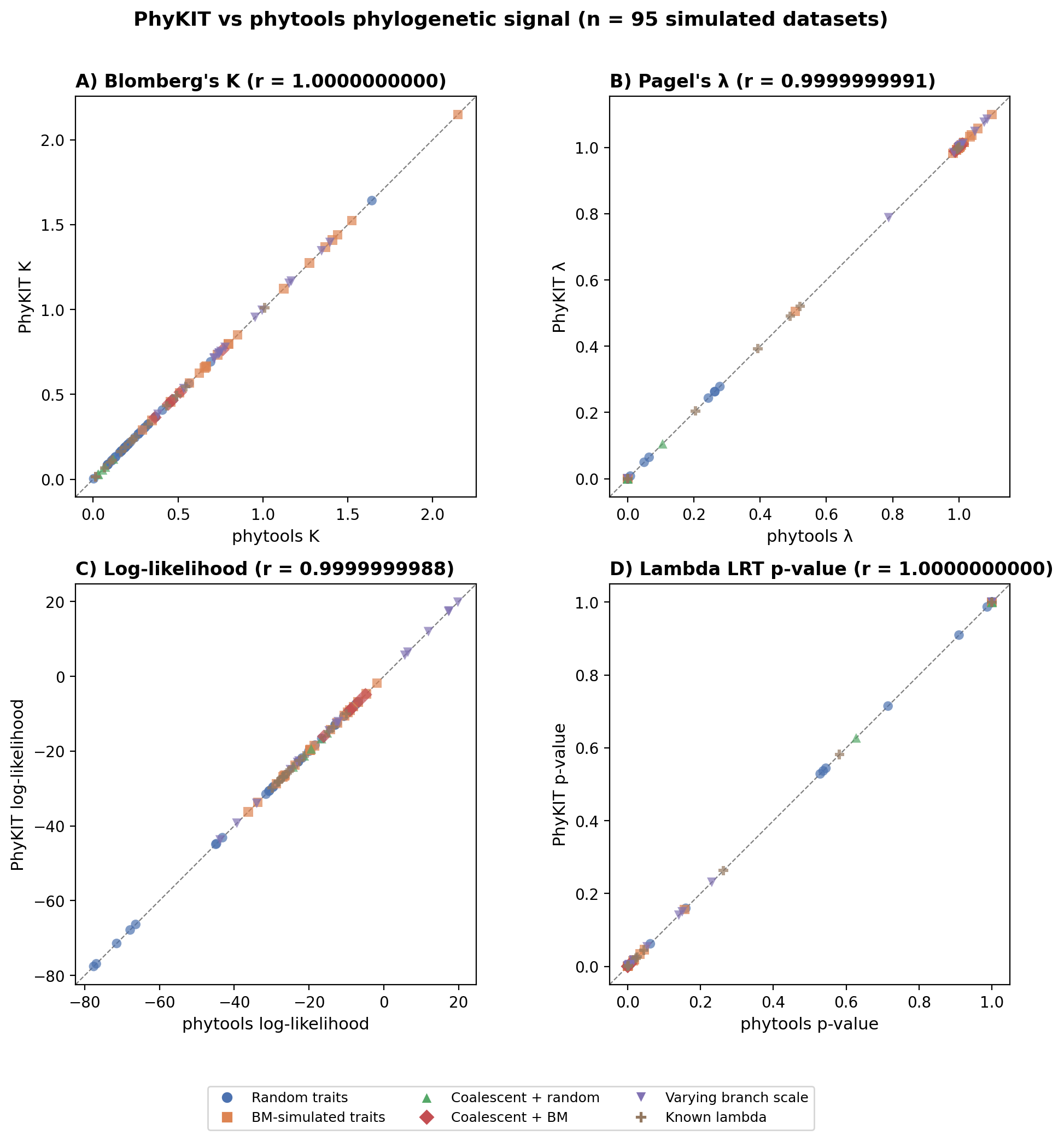
phykit phylogenetic_signal -t <tree> -d <trait_data> [-m <method>] [-p <permutations>] [-g <gene_trees>] [--multivariate] [--json]
Options:
-t/--tree: a tree file in Newick format
-d/--trait_data: tab-delimited trait file (taxon_name<tab>trait_value)
-m/--method: method to use: blombergs_k or lambda (default: blombergs_k)
-p/--permutations: number of permutations for Blomberg's K (default: 1000)
-g/--gene-trees: optional multi-Newick file of gene trees; when provided, uses a discordance-aware VCV (genome-wide average) instead of the species-tree VCV
--multivariate: compute K_mult (Adams 2014) for multivariate traits; the trait file should be a multi-column TSV with header row instead of two-column
--json: optional argument to print results as JSON
R validation: Validated against phytools, geiger in R
(see tests/r_validation/validate_signal_r2.R and tests/r_validation/validate_kmult.R).
Phylomorphospace
Function names: phylomorphospace; phylomorpho; phmo
Command line interface: pk_phylomorphospace; pk_phylomorpho; pk_phmo
Plot a phylomorphospace: two raw traits in trait space with the phylogeny
overlaid via ML-reconstructed ancestral states at internal nodes. This differs
from the phylogenetic_ordination --plot-tree option, which plots in PC space;
phylomorphospace plots raw trait values directly on the x and y axes.
Tree edges connect species through ML-reconstructed ancestral states and are
colored by distance from root (coolwarm colormap with colorbar). Tip points
default to blue, or can be colored by a continuous or discrete variable using
the --color-by option.
The multi-trait input file should be tab-delimited with a header row:
taxon<tab>trait1<tab>trait2<tab>...
Lines starting with '#' are treated as comments. If the tree and trait file
have different taxa, the intersection is used and warnings are printed to
stderr.
If the trait file has exactly 2 trait columns and --trait-x / --trait-y
are omitted, the first two columns are selected automatically.
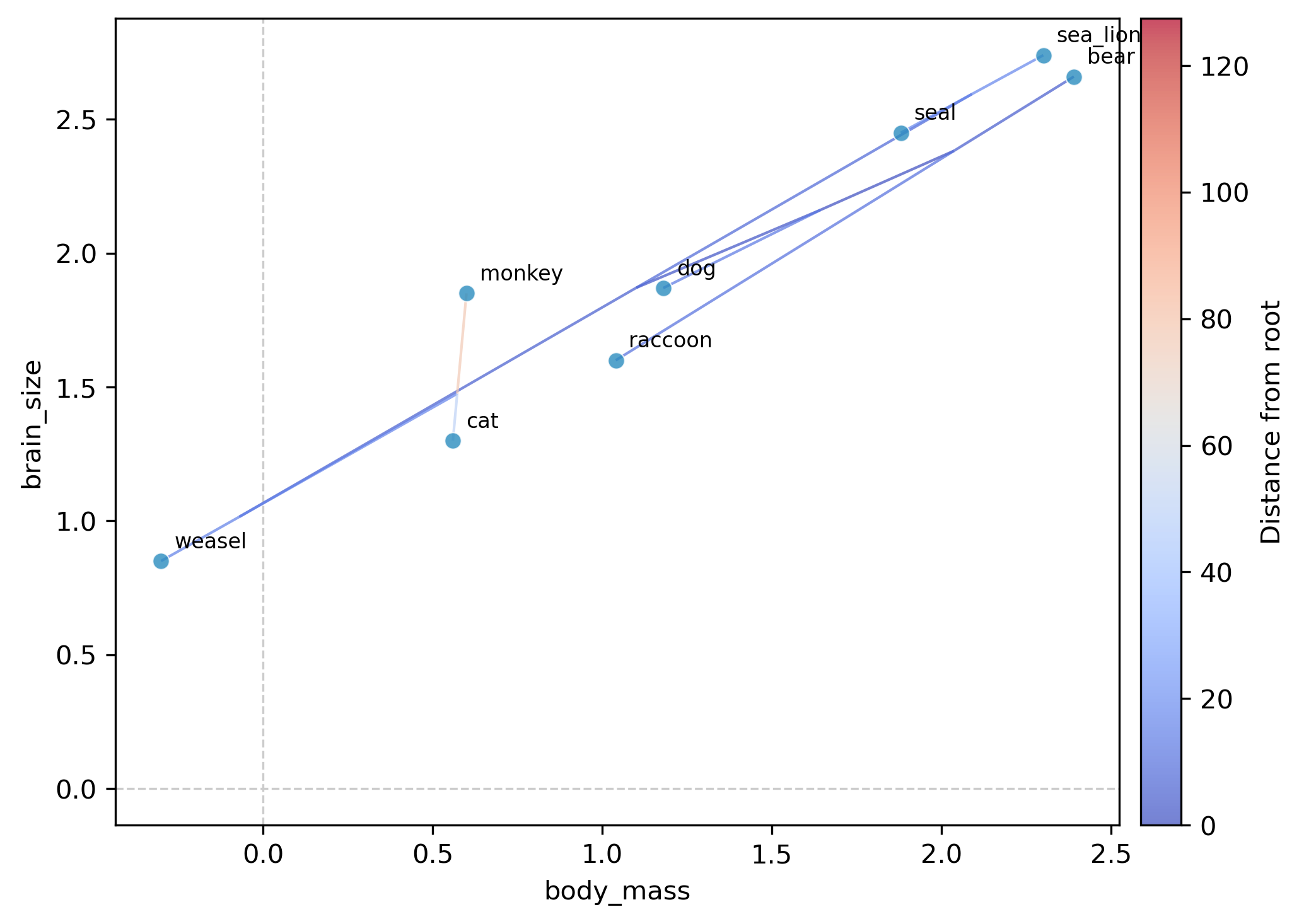
phykit phylomorphospace -t <tree> -d <trait_data> [--trait-x <name>] [--trait-y <name>] [--color-by <col_or_file>] [--plot-output <path>]
    [--fig-width <float>] [--fig-height <float>] [--dpi <int>] [--no-title] [--title <str>]
    [--legend-position <str>] [--ylabel-fontsize <float>] [--xlabel-fontsize <float>]
    [--title-fontsize <float>] [--axis-fontsize <float>] [--colors <str>] [--ladderize] [--cladogram] [--circular] [--color-file <file>] [--json]
Options:
-t/--tree: a tree file in Newick format
-d/--trait_data: tab-delimited multi-trait file with header row
--trait-x: column name for x-axis trait
--trait-y: column name for y-axis trait
--color-by: color tip points by a trait; specify a column name from the multi-trait file or a separate tab-delimited file (taxon<tab>value) for continuous or discrete coloring
--plot-output: output path for plot (default: phylomorphospace_plot.png)
--fig-width: figure width in inches (auto-scaled if omitted)
--fig-height: figure height in inches (auto-scaled if omitted)
--dpi: resolution in DPI (default: 300)
--no-title: hide the plot title
--title: custom title text
--legend-position: legend location (e.g., "upper right", "none" to hide)
--ylabel-fontsize: font size for y-axis labels; 0 to hide
--xlabel-fontsize: font size for x-axis labels; 0 to hide
--title-fontsize: font size for the title
--axis-fontsize: font size for axis labels
--colors: comma-separated colors (hex or named)
--ladderize: ladderize (sort) the tree before plotting
--cladogram: draw cladogram (equal branch lengths, tips aligned) instead of phylogram
--circular: draw circular (radial/fan) phylogram instead of rectangular
--color-file: color annotation file for tip labels, clade ranges, and branch colors (iTOL-inspired TSV format)
--json: optional argument to print results as JSON
Polytomy testing
Function names: polytomy_test; polyt_test; polyt; ptt
Command line interface: pk_polytomy_test; pk_polyt_test; pk_polyt; pk_ptt
Conduct a polytomy test for three clades in a phylogeny.
Polytomy tests can be used to identify putative radiations as well as identify well supported alternative topologies.
The polytomy testing function takes as input a file with the three groups of taxa to test the relationships for and a single column file with the names of the desired tree files to use for polytomy testing. Next, the script examines support for the grouping of the three taxa using triplets and gene support frequencies.
This function can account for uncertainty in gene trees - that is, the input phylogenies can have collapsed bipartitions.
Thereafter, a chi-squared test is conducted to determine if there is evidence to reject the null hypothesis wherein the null hypothesis is that the three possible topologies among the three groups are equally supported. This test is done using gene support frequencies.
phykit polytomy_test -t/--trees <trees> -g/--groups <groups> [--json]
Options:
-t/--trees <trees>: single column file with the names of
phylogenies to use for polytomy testing
-g/--groups: a tab-delimited file with the grouping designations
to test. Lines starting with comments are not considered. Names of
individual taxa should be separated by a semi-colon ';'
--json: optional argument to print results as JSON
For example, the groups file could look like the following:
#label group0  group1  group2
name_of_test    tip_name_A;tip_name_B   tip_name_C  tip_name_D;tip_name_E
Print tree
Function names: print_tree; print; pt
Command line interface: pk_print_tree; pk_print; pk_pt
Print ascii tree of input phylogeny.
Phylogeny can be printed with or without branch lengths. By default, the phylogeny will be printed with branch lengths but branch lengths can be removed using the -r/--remove argument.
phykit print_tree <tree> [-r/--remove] [--json]
Options:
<tree>: first argument after function name should be a tree file
-r/--remove: optional argument to print the phylogeny without branch
lengths
--json: optional argument to print results as JSON
Prune tree
Function names: prune_tree; prune
Command line interface: pk_prune_tree; pk_prune
Prune tips from a phylogeny.
Provide a single column file with the names of the tips in the input phylogeny you would like to prune from the tree.
phykit prune_tree <tree> <list_of_taxa> [-o/--output <output_file>] [-k/--keep]
    [--ignore-branch-labels] [--json]
Options:
<tree>: first argument after function name should be a tree file
<list_of_taxa>: single column file with the names of the tips to remove
from the phylogeny
-o/--output: name of output file for the pruned phylogeny.
Default output will have the same name as the input file but with the suffix
".pruned"
-k/--keep: optional argument. If used instead of pruning taxa in <list_of_taxa>,
keep them
--ignore-branch-labels: optional argument. Strip HyPhy/aBSREL-style {...}
branch labels (e.g., Hydlep{FG}) from tip names when matching against
<list_of_taxa>. The labels are preserved on the surviving tips in the
output tree, so a list of bare names produced by tools like seqkit seq -n
will keep (or remove) the foreground-tagged tips intact.
--json: optional argument to print results as JSON
Tip: when preparing trees for branch-site selection tests such as aBSREL or
RELAX, use --ignore-branch-labels together with -k to subset a labeled
species tree to the taxa present in a given orthogroup alignment without
losing the {FG} (foreground) annotations on the labeled branches.
Quartet network
Function names: quartet_network; quartet_net; qnet; nanuq
Command line interface: pk_quartet_network; pk_quartet_net; pk_qnet; pk_nanuq
Quartet-based network inference (NANUQ-style) for distinguishing incomplete lineage sorting (ILS) from hybridization/gene flow using quartet concordance factors from gene trees.
For each 4-taxon subset, counts how many gene trees display each of the 3 possible unrooted topologies and applies two hypothesis tests:
Star test (Pearson chi-squared): tests whether the three topology counts are consistent with a star tree (equal probabilities 1/3 each). If p_star > beta (default 0.95), the quartet is classified as unresolved.
T3 tree model test (G-test / likelihood ratio): tests whether the counts are consistent with any resolved quartet tree under the multispecies coalescent. If p_tree > alpha (default 0.05), the quartet is classified as tree-like (conflict is due to ILS).
If both tests reject their null hypotheses, the quartet is classified as hybrid (asymmetric discordance indicating gene flow or hybridization).
This algorithm matches the NANUQ method of Allman, Baños & Rhodes (2019), implemented in R's MSCquartets package.
Polytomies (collapsed branches) in gene trees are handled conservatively: bipartitions from polytomous nodes are excluded, so quartets spanning a polytomy are treated as unresolved rather than misclassified. Trifurcating roots (standard unrooted Newick) are not affected. This allows gene trees with collapsed low-support branches to be used directly as input.
Input can be either: 1) a file with one Newick tree per line, or 2) a file with one tree-file path per line.
phykit quartet_network -t/--trees <trees> [--alpha 0.05] [--beta 0.95] [--missing-taxa error|shared] [--plot-output <file>]
    [--fig-width <float>] [--fig-height <float>] [--dpi <int>] [--no-title] [--title <str>]
    [--legend-position <str>] [--ylabel-fontsize <float>] [--xlabel-fontsize <float>]
    [--title-fontsize <float>] [--axis-fontsize <float>] [--colors <str>] [--ladderize] [--cladogram] [--circular] [--color-file <file>] [--json]
Options:
-t/--trees: file containing trees (one Newick per line) or tree-file paths (one per line)
--alpha: significance level for the T3 tree model test (default: 0.05)
--beta: threshold for the star tree test; quartets with p_star > beta are called unresolved (default: 0.95)
--missing-taxa: handling strategy for mismatched taxa (error or shared; default: error)
--plot-output: output filename for the quartet network plot (optional)
--fig-width: figure width in inches (auto-scaled if omitted)
--fig-height: figure height in inches (auto-scaled if omitted)
--dpi: resolution in DPI (default: 300)
--no-title: hide the plot title
--title: custom title text
--legend-position: legend location (e.g., "upper right", "none" to hide)
--ylabel-fontsize: font size for y-axis labels; 0 to hide
--xlabel-fontsize: font size for x-axis labels; 0 to hide
--title-fontsize: font size for the title
--axis-fontsize: font size for axis labels
--colors: comma-separated colors (hex or named)
--ladderize: ladderize (sort) the tree before plotting
--cladogram: draw cladogram (equal branch lengths, tips aligned) instead of phylogram
--circular: draw circular (radial/fan) phylogram instead of rectangular
--color-file: color annotation file for tip labels, clade ranges, and branch colors (iTOL-inspired TSV format)
--json: optional argument to print results as JSON
When --plot-output is specified, a NANUQ-style splits graph is drawn from
the quartet distance matrix using Neighbor-Joining and circular split
decomposition. Tree-like relationships appear as simple branching, while
hybridization / reticulation produces characteristic box (parallelogram)
structures — the same style of output produced by R's MSCquartets +
NeighborNet pipeline.
No hybridization signal — all quartets are tree-like, so the splits graph is a clean unrooted tree:
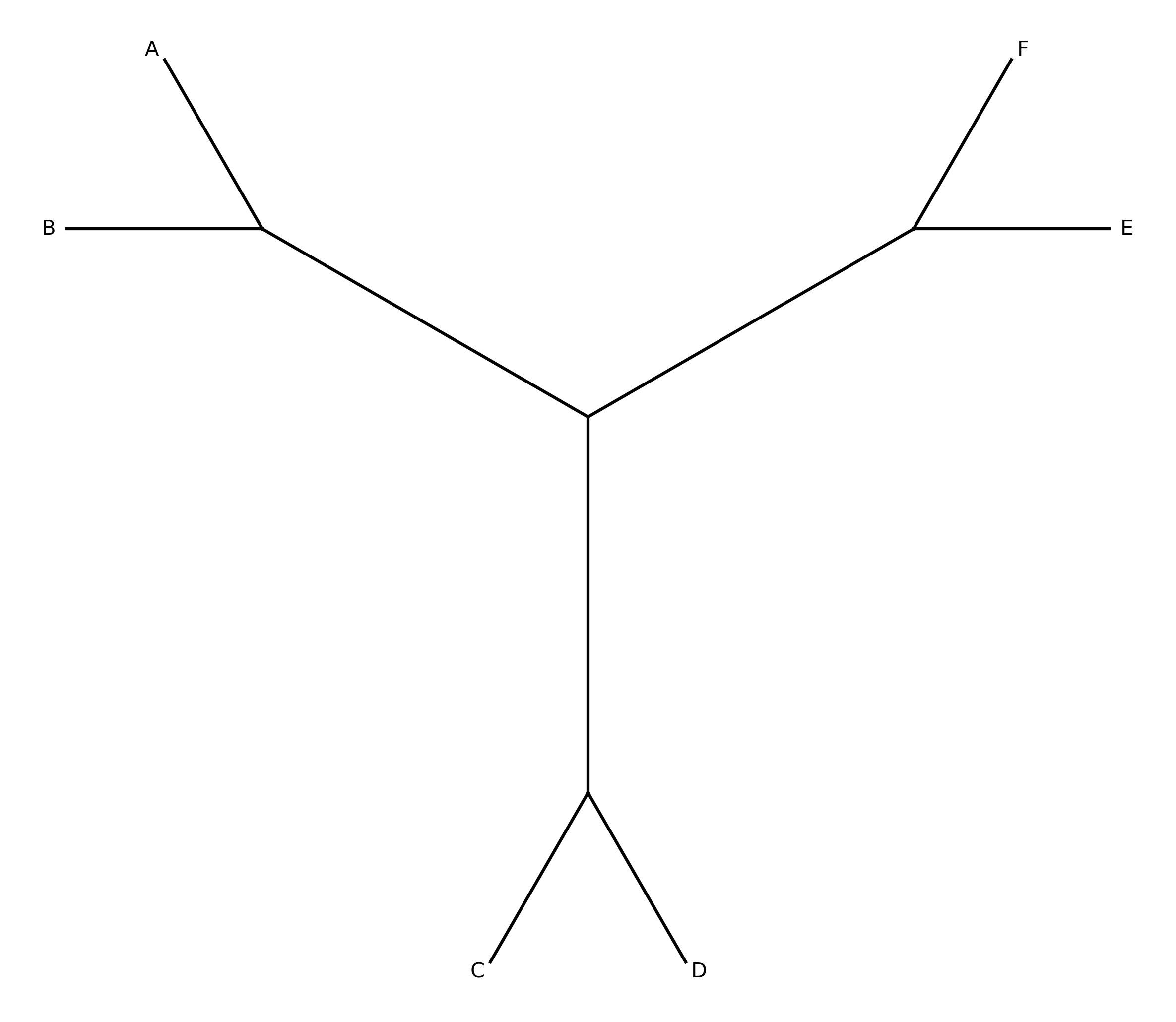
Hybridization signal present — hybrid quartets introduce conflicting splits that appear as boxes in the network, indicating reticulation among C, D, E, and F:
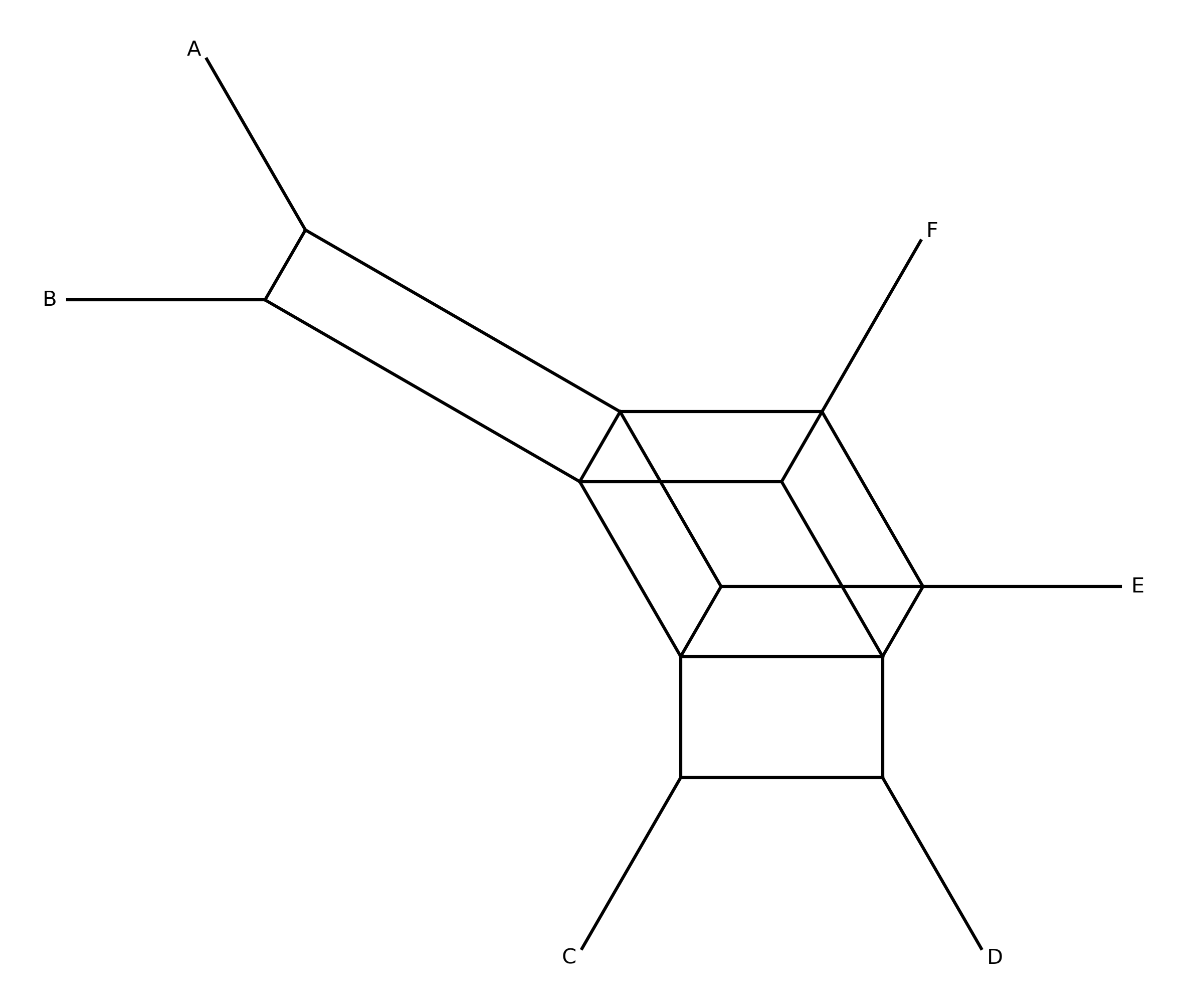
Quartet pie chart
Function names: quartet_pie; qpie; quartet_pie_chart
Command line interface: pk_quartet_pie; pk_qpie; pk_quartet_pie_chart
Draw a phylogram with pie charts at internal nodes showing quartet
concordance proportions. In native mode (-g provided), computes gene
concordance factors (gCF, gDF1, gDF2) from a species tree and gene trees
via bipartition matching. In ASTRAL mode (no -g), parses q1/q2/q3
annotations from ASTRAL -t 2 or wASTRAL --support 3 output.
Pie slices show concordant (blue), discordant alt 1 (red), and
discordant alt 2 (gray) proportions. Use --annotate to add numeric
values near each pie.
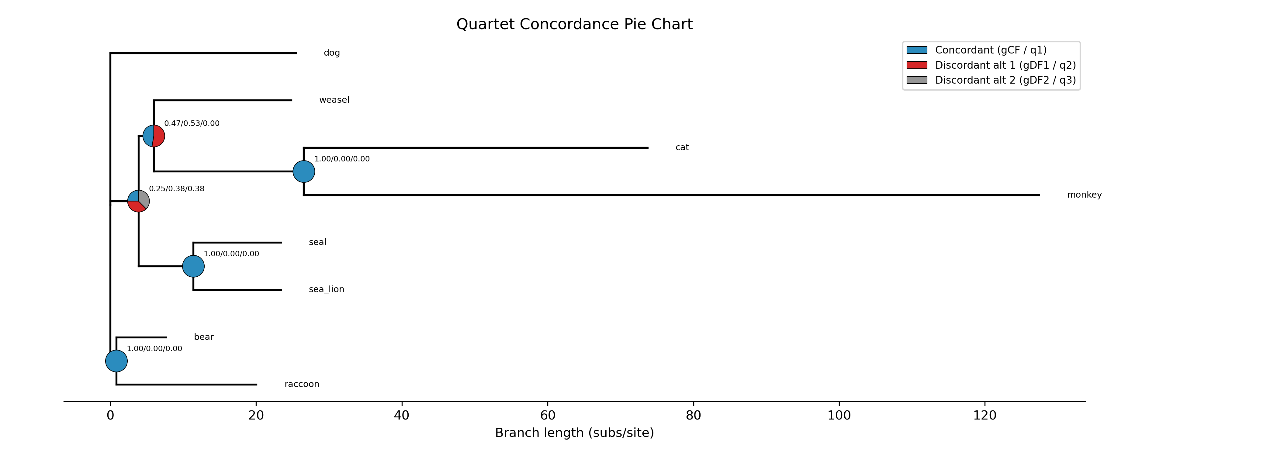
phykit quartet_pie -t <species_tree> [-g <gene_trees>] -o <output>
        [--annotate] [--branch-labels] [--csv <file>] [--ladderize] [--cladogram] [--circular] [--color-file <file>] [--json]
Options:
-t/--tree: species tree file (required)
-g/--gene-trees: gene trees file, one Newick tree per line (optional; if omitted, ASTRAL -t 2 or wASTRAL --support 3 annotations are parsed)
-o/--output: output figure path (required; supports .png, .pdf, .svg)
--annotate: show gCF/gDF values as text near each pie chart
--branch-labels: show the number of concordant gene trees (blue, above branch) and LPP support (red, below branch) on each internal branch. In ASTRAL mode, values come from f1 and pp1 annotations; in native mode, the concordant count is computed from gene trees
--csv: output per-branch concordance values (gCF, gDF1, gDF2, counts) as a CSV file
--pie-size: scale factor for pie chart size (default: 1.0; use 2.0 for double, 0.5 for half)
--colors: comma-separated colors for concordant, disc1, disc2 (default: blue, red, gray)
--ladderize: ladderize (sort) the tree before plotting
--cladogram: draw cladogram (equal branch lengths, tips aligned) instead of phylogram
--circular: draw circular (radial/fan) phylogram instead of rectangular
--color-file: color annotation file for tip labels, clade ranges, and branch colors (iTOL-inspired TSV format)
--json: optional argument to output per-node concordance values as JSON
Rate heterogeneity test (multi-rate Brownian motion)
Function names: rate_heterogeneity; brownie; rh
Command line interface: pk_rate_heterogeneity; pk_brownie; pk_rh
Test for rate heterogeneity across phylogenetic regimes using multi-rate
Brownian motion (O'Meara et al. 2006), analogous to R's
phytools::brownie.lite().
Fits single-rate vs. multi-rate BM models and performs a likelihood ratio
test. Users specify a tree, continuous trait data, and a regime file
mapping tips to regimes (tab-delimited, taxon<tab>regime_label).
Regime assignments to internal branches are inferred via Fitch parsimony. Per-regime VCV matrices are decomposed and per-regime sigma-squared values are estimated via maximum likelihood.
Optionally, a parametric bootstrap can be run to compute a simulated
p-value (-n/--nsim). A horizontal phylogram with branches colored by
regime can be generated using --plot.
An effect size metric R²_regime is also reported, measuring the variance reduction from regime-specific rates vs. a single rate, weighted by the number of tips per regime.
phykit rate_heterogeneity -t <tree> -d <trait_data> -r <regime_data> [-n <nsim>] [--seed <seed>] [--plot <output.png>]
    [--fig-width <float>] [--fig-height <float>] [--dpi <int>] [--no-title] [--title <str>]
    [--legend-position <str>] [--ylabel-fontsize <float>] [--xlabel-fontsize <float>]
    [--title-fontsize <float>] [--axis-fontsize <float>] [--colors <str>] [--ladderize] [--cladogram] [--circular] [--color-file <file>] [--json]
Options:
-t/--tree: a tree file in Newick format
-d/--trait_data: tab-delimited trait file (taxon<tab>value)
-r/--regime_data: tab-delimited regime file (taxon<tab>regime_label)
-n/--nsim: number of parametric bootstrap simulations (default: 0)
--seed: random seed for reproducibility
--plot: output plot file path for phylogram with colored branches
--fig-width: figure width in inches (auto-scaled if omitted)
--fig-height: figure height in inches (auto-scaled if omitted)
--dpi: resolution in DPI (default: 300)
--no-title: hide the plot title
--title: custom title text
--legend-position: legend location (e.g., "upper right", "none" to hide)
--ylabel-fontsize: font size for y-axis labels; 0 to hide
--xlabel-fontsize: font size for x-axis labels; 0 to hide
--title-fontsize: font size for the title
--axis-fontsize: font size for axis labels
--colors: comma-separated colors (hex or named)
--ladderize: ladderize (sort) the tree before plotting
--cladogram: draw cladogram (equal branch lengths, tips aligned) instead of phylogram
--circular: draw circular (radial/fan) phylogram instead of rectangular
--color-file: color annotation file for tip labels, clade ranges, and branch colors (iTOL-inspired TSV format)
--json: optional argument to print results as JSON
R validation: Validated against phytools in R
(see tests/r_validation/validate_brownie_r2.R).
Rename tree tips
Function names: rename_tree_tips; rename_tree; rename_tips
Command line interface: pk_rename_tree_tips; pk_rename_tree; pk_rename_tips
Renames tips in a phylogeny.
Renaming tips will follow the scheme of a tab-delimited file wherein the first column is the current tip name and the second column is the desired tip name in the resulting phylogeny.
phykit rename_tree_tips <tree> -i/--idmap <idmap.txt> [-o/--output <output_file>] [--json]
Options:
<tree>: first argument after function name should be a tree file
-i/--idmap: identifier map of current tip names (col1) and desired
tip names (col2)
-o/--output: optional argument to write the renamed tree files to. Default
output will have the same name as the input file but with the suffix ".renamed"
--json: optional argument to print results as JSON
Robinson-Foulds distance
Function names: robinson_foulds_distance; rf_distance; rf_dist; rf
Command line interface: pk_robinson_foulds_distance; pk_rf_distance; pk_rf_dist; pk_rf
Calculate Robinson-Foulds (RF) distance between two trees.
Low RF distances reflect greater similarity between two phylogenies. This function prints out two values, the plain RF value and the normalized RF value, which are separated by a tab. Normalized RF values are calculated by taking the plain RF value and dividing it by 2(n-3) where n is the number of tips in the phylogeny. Prior to calculating an RF value, PhyKIT will first determine the number of shared tips between the two input phylogenies and prune them to a common set of tips. Thus, users can input trees with different topologies and infer an RF value among subtrees with shared tips.
PhyKIT will print out col 1: the plain RF distance and col 2: the normalized RF distance.
RF distances are calculated following Robinson & Foulds, Mathematical Biosciences (1981), doi: 10.1016/0025-5564(81)90043-2.
phykit robinson_foulds_distance <tree_file_zero> <tree_file_one> [--json]
Options:
<tree_file_zero>: first argument after function name should be a tree file
<tree_file_one>: second argument after function name should be a tree file
--json: optional argument to print results as JSON
Root tree
Function names: root_tree; root; rt
Command line interface: pk_root_tree; pk_root; pk_rt
Roots phylogeny using user-specified taxa.
A list of taxa to root the phylogeny on should be specified using the -r argument. The root_taxa file should be a single-column file with taxa names. The output file will have the same name as the input tree file but with the suffix ".rooted".
phykit root_tree <tree> -r/--root <root_taxa> [-o/--output <output_file>] [--json]
Options:
<tree>: first argument after function name should be a tree file to root
-r/--root: single column file with taxa names to root the phylogeny on
-o/--output: optional argument to specify the name of the output file
--json: optional argument to print results as JSON
SIMMAP summary
Function names: simmap_summary; smsummary; describe_simmap
Command line interface: pk_simmap_summary; pk_smsummary; pk_describe_simmap
Run N stochastic character maps (SIMMAP) and summarize the results
per branch, analogous to phytools::describe.simmap() in R.
For each branch, reports:
Dwelling time proportions: the average fraction of time spent in each character state across all simulations
Expected transitions: the mean number of state changes on that branch
For each internal node, reports:
Posterior probabilities: the proportion of simulations in which each state was sampled at that node
Interpreting the output:
A branch with dwelling proportions
carnivore=0.72, herbivore=0.17,
omnivore=0.11
spent 72% of its evolutionary time in the carnivore state (averaged across N maps). This indicates high confidence the lineage was carnivorous along that branch.A node with posteriors
carnivore=0.56, herbivore=0.25, omnivore=0.19was reconstructed as carnivore in 56% of simulations. Low values across all states indicate genuine ancestral uncertainty.E[trans]is the expected number of state changes on each branch. High values on long branches are expected. Values > 1 on short branches suggest rapid trait evolution.
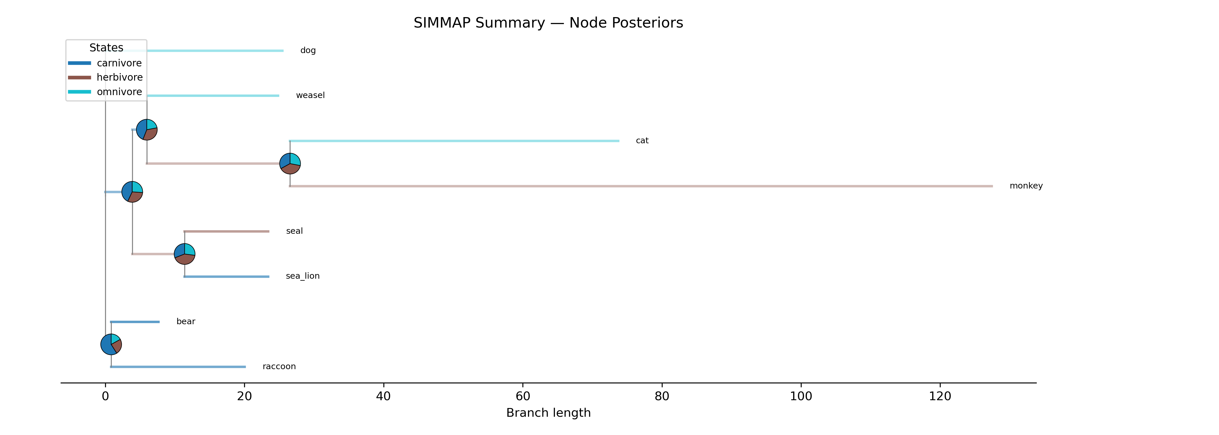
Tree with pie charts at internal nodes showing posterior state probabilities from 100 stochastic maps. Branches colored by the dominant state.
phykit simmap_summary -t <tree> -d <trait_data> -c <trait>
    [-m/--model ER|SYM|ARD] [-n/--nsim <int>]
    [--seed <int>] [--plot <file>] [--csv <file>] [--json]
Options:
-t/--tree: phylogenetic tree file (required)
-d/--trait_data: tab-delimited trait file with header row (required)
-c/--trait: column name for the discrete character trait (required)
-m/--model: substitution model — ER (equal rates, default), SYM (symmetric), or ARD (all rates different)
-n/--nsim: number of stochastic maps to simulate (default: 100)
--seed: random seed for reproducibility
--plot: output plot file showing tree with posterior pie charts at nodes (.png, .pdf, .svg)
--csv: output CSV file with per-branch dwelling proportions and node posteriors
--json: output results as JSON
R validation: Q matrix and log-likelihood validated against
phytools::fitMk() and phytools::make.simmap()
(see tests/r_validation/validate_simmap_summary.R).
Spectral discordance decomposition
Function names: spectral_discordance; spec_disc; sd
Command line interface: pk_spectral_discordance; pk_spec_disc; pk_sd
Decompose gene tree space via PCA on a bipartition presence/absence (or branch-length) matrix, with spectral clustering and automatic cluster detection via the eigengap heuristic.
Each gene tree is encoded as a vector over the union of all observed bipartitions. PCA reveals the axes of topological variation, with loading vectors directly identifying which bipartitions drive each PC. Spectral clustering groups genes sharing similar topologies; the number of clusters is auto-detected from the eigengap of the graph Laplacian.
Two metrics are available:
nrf (default): binary presence/absence, consistent with normalized Robinson-Foulds distance
wrf: branch-length weighted
Polytomies (collapsed branches) in gene trees are handled conservatively: splits from polytomous nodes are excluded from the bipartition matrix since they represent unresolved relationships. Trifurcating roots (standard unrooted Newick) are not affected. This allows gene trees with collapsed low-support branches to be used directly as input.
phykit spectral_discordance -g <gene_trees> [-t <tree>] [--metric nrf|wrf] [--clusters K] [--n-pcs N] [--top-loadings N] [--plot <prefix>]
    [--fig-width <float>] [--fig-height <float>] [--dpi <int>] [--no-title] [--title <str>]
    [--legend-position <str>] [--ylabel-fontsize <float>] [--xlabel-fontsize <float>]
    [--title-fontsize <float>] [--axis-fontsize <float>] [--colors <str>] [--ladderize] [--cladogram] [--circular] [--color-file <file>] [--json]
Options:
-g/--gene-trees: file of gene trees (one Newick per line, or file of filenames)
-t/--tree: species tree (optional; flags species-tree bipartitions in loadings)
--metric: distance metric: nrf or wrf (default: nrf)
--clusters: override auto-detected number of clusters
--n-pcs: number of PCs to report (default: min(10, G-1))
--top-loadings: top bipartitions per PC to display (default: 5)
--plot: output prefix for plots (generates _scatter.png and _eigengap.png)
--fig-width: figure width in inches (auto-scaled if omitted)
--fig-height: figure height in inches (auto-scaled if omitted)
--dpi: resolution in DPI (default: 300)
--no-title: hide the plot title
--title: custom title text
--legend-position: legend location (e.g., "upper right", "none" to hide)
--ylabel-fontsize: font size for y-axis labels; 0 to hide
--xlabel-fontsize: font size for x-axis labels; 0 to hide
--title-fontsize: font size for the title
--axis-fontsize: font size for axis labels
--colors: comma-separated colors (hex or named)
--ladderize: ladderize (sort) the tree before plotting
--cladogram: draw cladogram (equal branch lengths, tips aligned) instead of phylogram
--circular: draw circular (radial/fan) phylogram instead of rectangular
--color-file: color annotation file for tip labels, clade ranges, and branch colors (iTOL-inspired TSV format)
--json: output results as JSON
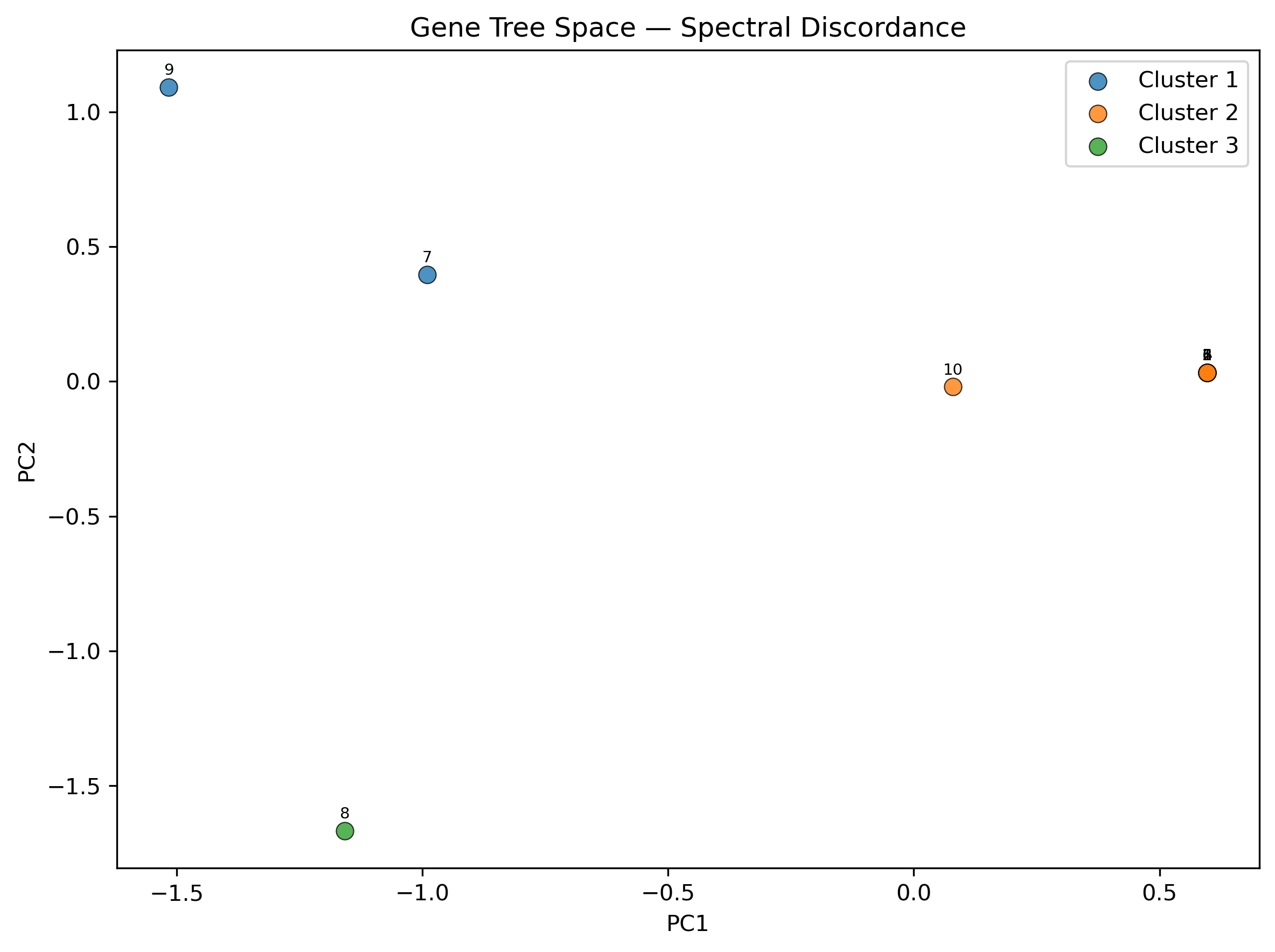
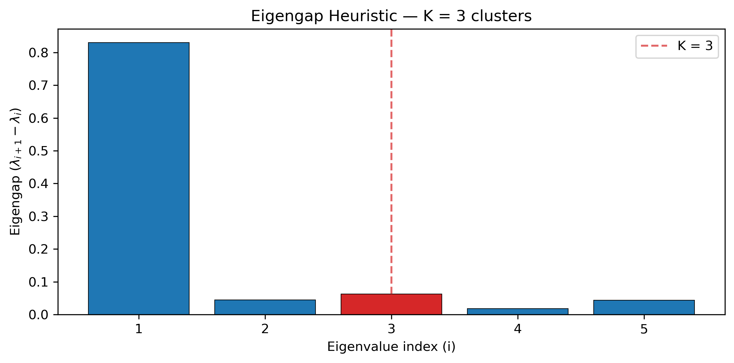
Spurious homolog identification
Function names: spurious_sequence; spurious_seq; ss
Command line interface: pk_spurious_sequence; pk_spurious_seq; pk_ss
Determines potentially spurious homologs using branch lengths.
Identifies potentially spurious sequences and reports tips in the phylogeny that could possibly be removed from the associated multiple sequence alignment. PhyKIT does so by identifying and reporting long terminal branches defined as branches that are equal to or greater than 20 times the median length of all branches.
PhyKIT reports the following information col1: name of tip that is a putatively spurious sequence col2: length of branch leading to putatively spurious sequence col3: threshold used to identify putatively spurious sequences col4: median branch length in the phylogeny
If there are no putatively spurious sequences, "None" is reported.
Using this method to identify potentially spurious sequences was, to my knowledge, first introduced by Shen et al., (2018) Cell doi: 10.1016/j.cell.2018.10.023.
phykit spurious_seq <file> -f/--factor [--json]
Options:
<file>: first argument after function name should be a tree file
-f/--factor: factor to multiply median branch length by to calculate
the threshold of long branches. (Default: 20)
--json: optional argument to print results as JSON
Stochastic character mapping (SIMMAP)
Function names: stochastic_character_map; simmap; scm
Command line interface: pk_stochastic_character_map; pk_simmap; pk_scm
Perform Stochastic Character Mapping (SIMMAP) of discrete traits onto a
phylogeny (Huelsenbeck et al. 2003; Bollback 2006), analogous to R's
phytools::make.simmap().
Fits a continuous-time Markov chain (CTMC) rate matrix Q via maximum likelihood using Felsenstein's pruning algorithm. Three substitution models are available:
ER (equal rates): 1 free parameter
SYM (symmetric rates): k(k-1)/2 free parameters
ARD (all rates differ): k(k-1) free parameters
The input trait file should be tab-delimited with a header row:
taxon<tab>trait_column<tab>...
Lines starting with '#' are treated as comments. If the tree and trait file
have different taxa, the intersection is used and warnings are printed to
stderr.
Output includes the fitted Q matrix, log-likelihood, mean dwelling times, mean transition counts, and posterior probabilities at internal nodes.
Optionally, a horizontal phylogram plot with branches colored by mapped
character state can be generated using the --plot argument.
All results have been validated against R 4.4.0 using phytools::fitMk
and phytools::make.simmap. ER log-likelihoods match R to within 0.002
(both optimizers converge to the same flat plateau). For the ARD model,
PhyKIT's multi-start optimizer finds a slightly better local optimum
than R (loglik -8.38 vs -8.43). Dwelling times sum to total tree length
exactly, and Q matrix structural properties (rows sum to zero, model
nesting) are verified.
phykit stochastic_character_map -t <tree> -d <trait_data> -c <trait_column> [-m <model>] [-n <nsim>] [--seed <seed>] [--plot <output.png>]
    [--fig-width <float>] [--fig-height <float>] [--dpi <int>] [--no-title] [--title <str>]
    [--legend-position <str>] [--ylabel-fontsize <float>] [--xlabel-fontsize <float>]
    [--title-fontsize <float>] [--axis-fontsize <float>] [--colors <str>] [--ladderize] [--cladogram] [--circular] [--color-file <file>] [--json]
Options:
-t/--tree: a tree file in Newick format
-d/--trait_data: tab-delimited trait file with header row
-c/--trait: column name for discrete character trait
-m/--model: substitution model: ER, SYM, or ARD (default: ER)
-n/--nsim: number of stochastic mapping simulations (default: 100)
--seed: random seed for reproducibility
--plot: output plot file path for phylogram with colored branches
--fig-width: figure width in inches (auto-scaled if omitted)
--fig-height: figure height in inches (auto-scaled if omitted)
--dpi: resolution in DPI (default: 300)
--no-title: hide the plot title
--title: custom title text
--legend-position: legend location (e.g., "upper right", "none" to hide)
--ylabel-fontsize: font size for y-axis labels; 0 to hide
--xlabel-fontsize: font size for x-axis labels; 0 to hide
--title-fontsize: font size for the title
--axis-fontsize: font size for axis labels
--colors: comma-separated colors (hex or named)
--ladderize: ladderize (sort) the tree before plotting
--cladogram: draw cladogram (equal branch lengths, tips aligned) instead of phylogram
--circular: draw circular (radial/fan) phylogram instead of rectangular
--color-file: color annotation file for tip labels, clade ranges, and branch colors (iTOL-inspired TSV format)
--json: optional argument to print results as JSON
Subtree pruning and regrafting
Function names: subtree_prune_regraft; spr
Command line interface: pk_subtree_prune_regraft; pk_spr
Generate all possible SPR (Subtree Pruning and Regrafting) rearrangements for a specified subtree on a tree.
The subtree is identified by specifying one or more comma-separated taxa whose MRCA (most recent common ancestor) defines the clade to prune. The pruned subtree is then regrafted onto every other branch in the remaining tree, producing one Newick tree per regraft position.
For a subtree defined by a single taxon (a single leaf), the leaf is pruned and reattached to each branch in the remaining tree. For a clade (two or more taxa), the entire clade is pruned and regrafted. Each output Newick contains all original taxa.
phykit subtree_prune_regraft -t <tree> --subtree <taxa> [-o/--output <output_file>] [--json]
Options:
-t/--tree: input tree file in Newick format (required)
--subtree: comma-separated list of taxa defining the subtree to prune (MRCA resolved), or a single-column file with one taxon per line (required)
-o/--output: optional output file for SPR trees (one Newick per line); if omitted, prints to stdout
--json: optional argument to print summary metadata and trees as JSON
Terminal branch statistics
Function names: terminal_branch_stats; tbs
Command line interface: pk_terminal_branch_stats; pk_tbs
Calculate summary statistics for terminal branch lengths in a phylogeny.
Terminal branch lengths can be useful for phylogeny diagnostics.
To obtain all terminal branch lengths, use the -v/--verbose option.
phykit terminal_branch_stats <tree> [-v/--verbose] [--json]
Options:
<tree>: first argument after function name should be a tree file
-v/--verbose: optional argument to print all terminal branch lengths
--json: optional argument to print results as JSON
Threshold model
Function names: threshold_model; threshold; thresh; threshbayes; thresh_bayes
Command line interface: pk_threshold_model; pk_threshold; pk_thresh; pk_threshbayes; pk_thresh_bayes
Estimate the evolutionary correlation between two traits using the Felsenstein (2012) threshold model via MCMC. Binary discrete characters are modelled as arising from continuous latent "liabilities" that evolve under Brownian motion and cross a threshold at 0. This lets you estimate correlations between binary traits (or between a binary and a continuous trait) using BM rather than Mk transition rates.
This is the Python equivalent of phytools::threshBayes in R.
The sampler uses a Gibbs / Metropolis-Hastings hybrid:
Gibbs step: sample each discrete tip's liability from a truncated normal conditioned on all other values
Metropolis step: update sigma2_1, sigma2_2 (log-normal proposal), ancestral values a1, a2 (normal proposal), and the correlation r (normal proposal with reflection on [-1, 1])
Adaptive tuning: during burn-in, proposal variances are adjusted to target ~23% acceptance
Trait types:
discrete: binary (0/1). Liabilities < 0 map to state 0, liabilities > 0 map to state 1.continuous: observed values used directly (no liability needed).
Any combination of two traits is supported: discrete+continuous, discrete+discrete, or continuous+continuous.
phykit threshold_model -t <tree> -d <trait_data> --traits <t1,t2> --types <type1,type2> [--ngen 100000] [--sample 100] [--burnin 0.2] [--seed <int>] [--plot <file>]
    [--fig-width <float>] [--fig-height <float>] [--dpi <int>] [--no-title] [--title <str>]
    [--legend-position <str>] [--ylabel-fontsize <float>] [--xlabel-fontsize <float>]
    [--title-fontsize <float>] [--axis-fontsize <float>] [--colors <str>] [--ladderize] [--cladogram] [--circular] [--color-file <file>] [--json]
Options:
-t/--tree: a rooted phylogeny file with branch lengths (required)
-d/--trait-data: tab-delimited trait file with header row (required)
--traits: comma-separated pair of trait column names (required)
--types: comma-separated pair of trait types, each discrete or continuous (required)
--ngen: number of MCMC generations (default: 100000)
--sample: sample frequency (default: 100)
--burnin: burn-in fraction (default: 0.2)
--seed: random seed for reproducibility
--plot: output filename for trace and posterior density plot (3 rows x 2 columns:
left = MCMC trace, right = posterior histogram with 95% HPD shading)
--fig-width: figure width in inches (auto-scaled if omitted)
--fig-height: figure height in inches (auto-scaled if omitted)
--dpi: resolution in DPI (default: 300)
--no-title: hide the plot title
--title: custom title text
--legend-position: legend location (e.g., "upper right", "none" to hide)
--ylabel-fontsize: font size for y-axis labels; 0 to hide
--xlabel-fontsize: font size for x-axis labels; 0 to hide
--title-fontsize: font size for the title
--axis-fontsize: font size for axis labels
--colors: comma-separated colors (hex or named)
--ladderize: ladderize (sort) the tree before plotting
--cladogram: draw cladogram (equal branch lengths, tips aligned) instead of phylogram
--circular: draw circular (radial/fan) phylogram instead of rectangular
--color-file: color annotation file for tip labels, clade ranges, and branch colors (iTOL-inspired TSV format)
--json: optional argument to print results as JSON
Output (text mode):
Trait 1: habitat (discrete, 2 states: 0, 1)
Trait 2: body_mass (continuous)
MCMC: 100000 generations, sampled every 100, burn-in 20%
---
Posterior correlation (r): 0.6234 (95% HPD: 0.312, 0.891)
Posterior sigma2_1: 1.234 (95% HPD: 0.456, 2.345)
Posterior sigma2_2: 0.567 (95% HPD: 0.234, 1.012)
Acceptance rates: r=0.234, sigma2_1=0.312, sigma2_2=0.287, a1=0.241, a2=0.228
Tutorial: habitat type and body mass in carnivores
This example uses the classic 8-taxon carnivore tree to test whether habitat type (a binary trait: 0 = non-arboreal, 1 = arboreal) is correlated with body mass on the latent liability scale.
Step 1: Prepare the trait file.
Create a tab-delimited file with a header row. The first column is the taxon name, followed by columns for each trait:
taxon        habitat body_mass
raccoon      0       1.04
bear 0       2.39
sea_lion     0       2.30
seal 0       1.88
monkey       1       0.60
cat  1       0.56
weasel       1       -0.30
dog  0       1.18
Step 2: Run the threshold model.
phykit threshold_model \
  -t carnivore.tre \
  -d traits.tsv \
  --traits habitat,body_mass \
  --types discrete,continuous \
  --ngen 100000 \
  --seed 42
Step 3: Examine the trace plots for convergence.
phykit threshold_model \
  -t carnivore.tre \
  -d traits.tsv \
  --traits habitat,body_mass \
  --types discrete,continuous \
  --ngen 100000 \
  --seed 42 \
  --plot trace.png
This generates a 3-row x 2-column figure. The left column shows MCMC trace plots for r, sigma2_1, and sigma2_2 (check for stationarity and good mixing). The right column shows posterior density histograms with red shading for the 95% HPD interval and a dashed line at the posterior mean.
Step 4: Get full posterior samples as JSON for custom analysis.
phykit threshold_model \
  -t carnivore.tre \
  -d traits.tsv \
  --traits habitat,body_mass \
  --types discrete,continuous \
  --ngen 100000 \
  --seed 42 \
  --json > posterior.json
The JSON output includes full posterior sample arrays, summary statistics (mean, median, 95% HPD), and MCMC metadata.
Tip labels
Function names: tip_labels; tree_labels; labels; tl
Command line interface: pk_tip_labels; pk_tree_labels; pk_labels; pk_tl
Prints the tip labels (or names) of a phylogeny.
phykit tip_labels <tree> [--json]
Options:
<tree>: first argument after function name should be a tree file
--json: optional argument to print results as JSON
Tip-to-tip distance
Function names: tip_to_tip_distance; t2t_dist; t2t
Command line interface: pk_tip_to_tip_distance; pk_t2t_dist; pk_t2t
Calculate distance between two tips (or leaves) in a phylogeny.
Distances are in substitutions per site.
phykit tip_to_tip_distance <tree_file> <tip_1> <tip_2> [--json]
phykit tip_to_tip_distance <tree_file> --all-pairs [--plot] [--plot-output <path>]
    [--fig-width <float>] [--fig-height <float>] [--dpi <int>] [--no-title] [--title <str>]
    [--legend-position <str>] [--ylabel-fontsize <float>] [--xlabel-fontsize <float>]
    [--title-fontsize <float>] [--axis-fontsize <float>] [--colors <str>] [--ladderize] [--cladogram] [--circular] [--color-file <file>] [--json]
Options:
<tree_file>: first argument after function name should be a tree file
<tip_1>: second argument should be the name of the first tip of interest
<tip_2>: third argument should be the name of the second tip of interest
--all-pairs: optional argument to report all pairwise tip distances
--plot: optional argument to save a clustered distance heatmap (requires --all-pairs)
--plot-output: output path for heatmap (default: tip_to_tip_distance_heatmap.png)
--fig-width: figure width in inches (auto-scaled if omitted)
--fig-height: figure height in inches (auto-scaled if omitted)
--dpi: resolution in DPI (default: 300)
--no-title: hide the plot title
--title: custom title text
--legend-position: legend location (e.g., "upper right", "none" to hide)
--ylabel-fontsize: font size for y-axis labels; 0 to hide
--xlabel-fontsize: font size for x-axis labels; 0 to hide
--title-fontsize: font size for the title
--axis-fontsize: font size for axis labels
--colors: comma-separated colors (hex or named)
--ladderize: ladderize (sort) the tree before plotting
--cladogram: draw cladogram (equal branch lengths, tips aligned) instead of phylogram
--circular: draw circular (radial/fan) phylogram instead of rectangular
--color-file: color annotation file for tip labels, clade ranges, and branch colors (iTOL-inspired TSV format)
--json: optional argument to print results as JSON
Tip-to-tip node distance
Function names: tip_to_tip_node_distance; t2t_node_dist; t2t_nd
Command line interface: pk_tip_to_tip_node_distance; pk_t2t_node_dist; pk_t2t_nd
Calculate distance between two tips (or leaves) in a phylogeny.
Distance is measured by the number of nodes between one tip and another.
phykit tip_to_tip_node_distance <tree_file> <tip_1> <tip_2> [--json]
Options:
<tree_file>: first argument after function name should be a tree file
<tip_1>: second argument should be the name of the first tip of interest
<tip_2>: third argument should be the name of the second tip of interest
--json: optional argument to print results as JSON
Total tree length
Function names: total_tree_length; tree_len
Command line interface: pk_total_tree_length; pk_tree_len
Calculate total tree length, which is a sum of all branches.
phykit total_tree_length <tree> [--json]
Options:
<tree>: first argument after function name should be a tree file
--json: optional argument to print results as JSON
Trait correlation
Function names: trait_correlation; trait_corr; phylo_corr
Command line interface: pk_trait_correlation; pk_trait_corr; pk_phylo_corr
Compute phylogenetic correlations between all pairs of traits and display them as a heatmap with significance indicators.
Uses GLS-centering via the tree's variance-covariance matrix to account for phylogenetic non-independence among species. P-values are computed from the t-distribution and displayed as significance stars on the heatmap cells:
***p < 0.001**p < 0.01*p < alpha (default 0.05)
The multi-trait input file should be tab-delimited with a header row:
taxon<tab>trait1<tab>trait2<tab>...
At least 2 traits are required. Lines starting with '#' are treated as
comments. If the tree and trait file have different taxa, the intersection
is used and warnings are printed to stderr.
The --cluster option clusters traits by correlation similarity
(using 1 - |r| as distance) and draws dendrograms alongside the
heatmap.
phykit trait_correlation -t <tree> -d <trait_data> -o <output>
    [--alpha 0.05] [--cluster] [-g <gene_trees>] [--json]
    [--fig-width <float>] [--fig-height <float>] [--dpi <int>]
    [--no-title] [--title <str>]
Options:
-t/--tree: a tree file in Newick format
-d/--trait-data: tab-delimited multi-trait file with header row (at least 2 traits)
-o/--output: output figure path (supports .png, .pdf, .svg)
--alpha: significance threshold for marking p-values (default: 0.05)
--cluster: cluster traits by correlation similarity and display dendrograms
-g/--gene-trees: optional multi-Newick file of gene trees for discordance-aware VCV
--json: optional argument to print results as JSON
Trait rate map
Function names: trait_rate_map; rate_map; branch_rates
Command line interface: pk_trait_rate_map; pk_rate_map; pk_branch_rates
Estimate per-branch evolutionary rates for a continuous trait and
display them as a branch-colored phylogram. Ancestral states are
reconstructed via Felsenstein's weighted-average method. Per-branch
rate is the squared standardized contrast (proportional to local
Brownian motion rate): rate = (child_val - parent_val)^2 / branch_length.
phykit trait_rate_map -t <tree> -d <trait_data> -o <output>
    [--trait <column>] [--json]
    [--fig-width <float>] [--fig-height <float>] [--dpi <int>] [--no-title] [--title <str>]
    [--legend-position <str>] [--ylabel-fontsize <float>] [--xlabel-fontsize <float>]
    [--title-fontsize <float>] [--axis-fontsize <float>] [--colors <str>] [--ladderize] [--cladogram] [--circular] [--color-file <file>]
Options:
-t/--tree: a tree file in Newick format
-d/--trait_data: tab-delimited trait file (two-column: taxon<tab>value with no header; or multi-column with header when --trait is used)
-o/--output: output plot file path (required)
--trait: column name to use from a multi-column trait file (if omitted, two-column format is expected)
--fig-width: figure width in inches (auto-scaled if omitted)
--fig-height: figure height in inches (auto-scaled if omitted)
--dpi: resolution in DPI (default: 300)
--no-title: hide the plot title
--title: custom title text
--legend-position: legend location (e.g., "upper right", "none" to hide)
--ylabel-fontsize: font size for y-axis labels; 0 to hide
--xlabel-fontsize: font size for x-axis labels; 0 to hide
--title-fontsize: font size for the title
--axis-fontsize: font size for axis labels
--colors: comma-separated colors (hex or named)
--ladderize: ladderize (sort) the tree before plotting
--cladogram: draw cladogram (equal branch lengths, tips aligned) instead of phylogram
--circular: draw circular (radial/fan) phylogram instead of rectangular
--color-file: color annotation file for tip labels, clade ranges, and branch colors (iTOL-inspired TSV format)
--json: optional argument to print results as JSON
Transfer annotations
Function names: transfer_annotations; transfer_annot; annotate_tree
Command line interface: pk_transfer_annotations; pk_transfer_annot; pk_annotate_tree
Transfer internal node annotations from one tree onto another. Matches nodes by bipartition (the set of descendant taxa) and copies the annotation labels from the source to the target tree.
Typical use case: Transfer wASTRAL support annotations (q1/q2/q3,
pp1, f1, localPP, etc.) from a wASTRAL --support 3 output tree onto
a branch-length-optimized topology from RAxML-NG, IQ-TREE, or any other
tool. The output tree has the target's branch lengths with the source's
annotations, ready for use with quartet_pie or other visualization
tools.
This function works with any Newick node annotations — not just wASTRAL.
Any labels or comments attached to internal nodes in the source tree will
be transferred to the matching nodes in the target tree (e.g., ASTRAL
-t 2 annotations, bootstrap support values, Bayesian posterior
probabilities, or custom labels).
Workflow:
Run wASTRAL to get an annotated species tree (mode 1 or 4,
--support 3)Extract the unannotated s0 topology
Optimize branch lengths on s0 with RAxML-NG or IQ-TREE
Transfer annotations from step 1 onto the optimized tree from step 3:
phykit transfer_annotations \
    --source wastral_annotated.tre \
    --target raxml_optimized.tre \
    -o combined.tre

# Now use the combined tree with quartet_pie
phykit qpie -t combined.tre -o concordance.png --branch-labels
phykit transfer_annotations --source <annotated_tree> --target <branch_length_tree>
    [-o/--output <file>] [--json]
Options:
--source: annotated tree file, e.g., wASTRAL output with --support 3 or any tree with node labels/comments (required)
--target: target tree file with branch lengths to keep, e.g., RAxML-NG or IQ-TREE output (required)
-o/--output: output file for the annotated tree (default: target file + .annotated)
--json: output results as JSON
Tree space visualization
Function names: tree_space; tspace; tree_landscape
Command line interface: pk_tree_space; pk_tspace; pk_tree_landscape
Visualize how gene trees cluster in topology space by computing pairwise distances (Robinson-Foulds or Kuhner-Felsenstein) and projecting into 2D via MDS, t-SNE, or UMAP. Points are colored by spectral clustering with automatic cluster detection via the eigengap heuristic.
Alternatively, use --heatmap to draw a clustered distance heatmap
with a dendrogram showing hierarchical relationships among gene trees.
Use --distance-matrix to export the raw pairwise distance matrix
as a CSV file.
Optionally highlight a species tree as a distinct marker to see where it sits relative to the gene tree cloud.
phykit tree_space -t <trees> -o <output>
    [--metric rf|kf] [--method mds|tsne|umap]
    [--species-tree <file>] [--k <int>] [--seed <int>]
    [--heatmap] [--distance-matrix <file>]
    [--fig-width <float>] [--fig-height <float>] [--dpi <int>] [--no-title] [--title <str>]
    [--legend-position <str>] [--ylabel-fontsize <float>] [--xlabel-fontsize <float>]
    [--title-fontsize <float>] [--axis-fontsize <float>] [--colors <str>] [--ladderize] [--cladogram] [--circular] [--color-file <file>] [--json]
Options:
-t/--trees: file with gene trees (one Newick per line, or one file path per line) (required)
-o/--output: output figure path (.png, .pdf, .svg) (required)
--metric: distance metric: rf (normalized Robinson-Foulds, default) or kf (Kuhner-Felsenstein)
--method: dimensionality reduction: mds (default), tsne, or umap
--species-tree: optional species tree to highlight in the plot as a star marker
--k: number of clusters (auto-detected via eigengap if omitted)
--seed: random seed for reproducibility (t-SNE/UMAP)
--heatmap: draw a clustered distance heatmap instead of a scatter plot
--distance-matrix: output the pairwise distance matrix as a CSV file
--json: optional argument to print results as JSON
Treeness
Function names: treeness; tness
Command line interface: pk_treeness; pk_tness
Calculate treeness statistic for a phylogeny.
Higher treeness values are thought to be desirable because they represent a higher signal-to-noise ratio.
Treeness is the sum of internal branch lengths divided by the total tree length. Therefore, values range from 0 to 1. Treeness can be used as a measure of the signal-to-noise ratio in a phylogeny.
Calculate treeness (also referred to as stemminess) following Lanyon, The Auk (1988), doi: 10.1093/auk/105.3.565 and Phillips and Penny, Molecular Phylogenetics and Evolution (2003), doi: 10.1016/S1055-7903(03)00057-5.
phykit treeness <tree> [--json]
Options:
<tree>: first argument after function name should be a tree file
--json: optional argument to print results as JSON
Alignment- and tree-based functions
Relative rate test
Function names: relative_rate_test; rrt; tajima_rrt
Command line interface: pk_relative_rate_test; pk_rrt; pk_tajima_rrt
Tajima's relative rate test (Tajima, Genetics, 1993).
Tests whether two ingroup lineages have evolved at equal rates since diverging from their common ancestor. The outgroup is automatically inferred from the rooted tree as the earliest-diverging taxon (the single taxon on the smaller side of the root split). All pairwise ingroup combinations are tested with Bonferroni and Benjamini-Hochberg FDR multiple testing correction.
At each alignment column, the test classifies informative sites:
m1: the first ingroup taxon differs from the outgroup, but the second matches
m2: the second ingroup taxon differs from the outgroup, but the first matches
Sites where both differ or both match the outgroup are uninformative and skipped
Sites with gaps or ambiguous characters are skipped
Test statistic: chi2 = (m1 - m2)^2 / (m1 + m2), with 1 degree of freedom.
Single alignment mode:
phykit relative_rate_test -a <alignment> -t <rooted_tree> [-v/--verbose]
    [--plot-output <path>] [--fig-width <float>] [--fig-height <float>] [--dpi <int>]
    [--no-title] [--title <str>] [--legend-position <str>] [--ylabel-fontsize <float>]
    [--xlabel-fontsize <float>] [--title-fontsize <float>] [--axis-fontsize <float>]
    [--colors <str>] [--ladderize] [--cladogram] [--circular] [--color-file <file>] [--json]
Batch mode (multiple alignments, one shared tree):
phykit relative_rate_test -l <alignment_list> -t <rooted_tree> [-v/--verbose]
    [--plot-output <path>] [--fig-width <float>] [--fig-height <float>] [--dpi <int>]
    [--no-title] [--title <str>] [--legend-position <str>] [--ylabel-fontsize <float>]
    [--xlabel-fontsize <float>] [--title-fontsize <float>] [--axis-fontsize <float>]
    [--colors <str>] [--ladderize] [--cladogram] [--circular] [--color-file <file>] [--json]
Options:
-a/--alignment: a single alignment file
-l/--alignment-list: a file with one alignment path per line (batch mode)
-t/--tree: a rooted tree file
-v/--verbose: print additional detail
--plot-output: save a pairwise p-value heatmap to this path
--fig-width: figure width in inches (auto-scaled if omitted)
--fig-height: figure height in inches (auto-scaled if omitted)
--dpi: resolution in DPI (default: 300)
--no-title: hide the plot title
--title: custom title text
--legend-position: legend location (e.g., "upper right", "none" to hide)
--ylabel-fontsize: font size for y-axis labels; 0 to hide
--xlabel-fontsize: font size for x-axis labels; 0 to hide
--title-fontsize: font size for the title
--axis-fontsize: font size for axis labels
--colors: comma-separated colors (hex or named)
--ladderize: ladderize (sort) the tree before plotting
--cladogram: draw cladogram (equal branch lengths, tips aligned) instead of phylogram
--circular: draw circular (radial/fan) phylogram instead of rectangular
--color-file: color annotation file for tip labels, clade ranges, and branch colors (iTOL-inspired TSV format)
--json: optional argument to print results as JSON
Single mode outputs one row per ingroup pair with m1, m2, chi-squared, raw p-value, Bonferroni-corrected p-value, FDR-corrected p-value, and a significance indicator. Batch mode aggregates across genes, reporting the number and percentage of genes rejecting equal rates for each pair.
When --plot-output is provided, a symmetric heatmap of
-log10(FDR-corrected p-values) is saved. Cells with significant
pairs (FDR < 0.05) are marked with an asterisk. Darker colors
indicate stronger evidence for unequal evolutionary rates.
The dashed line on the colorbar marks the significance threshold
(-log10(0.05) ≈ 1.3); cells above this line are significant.
Equal rates — all taxa evolve at similar rates, so no pairwise comparison reaches significance. The heatmap is uniformly pale with no asterisks:
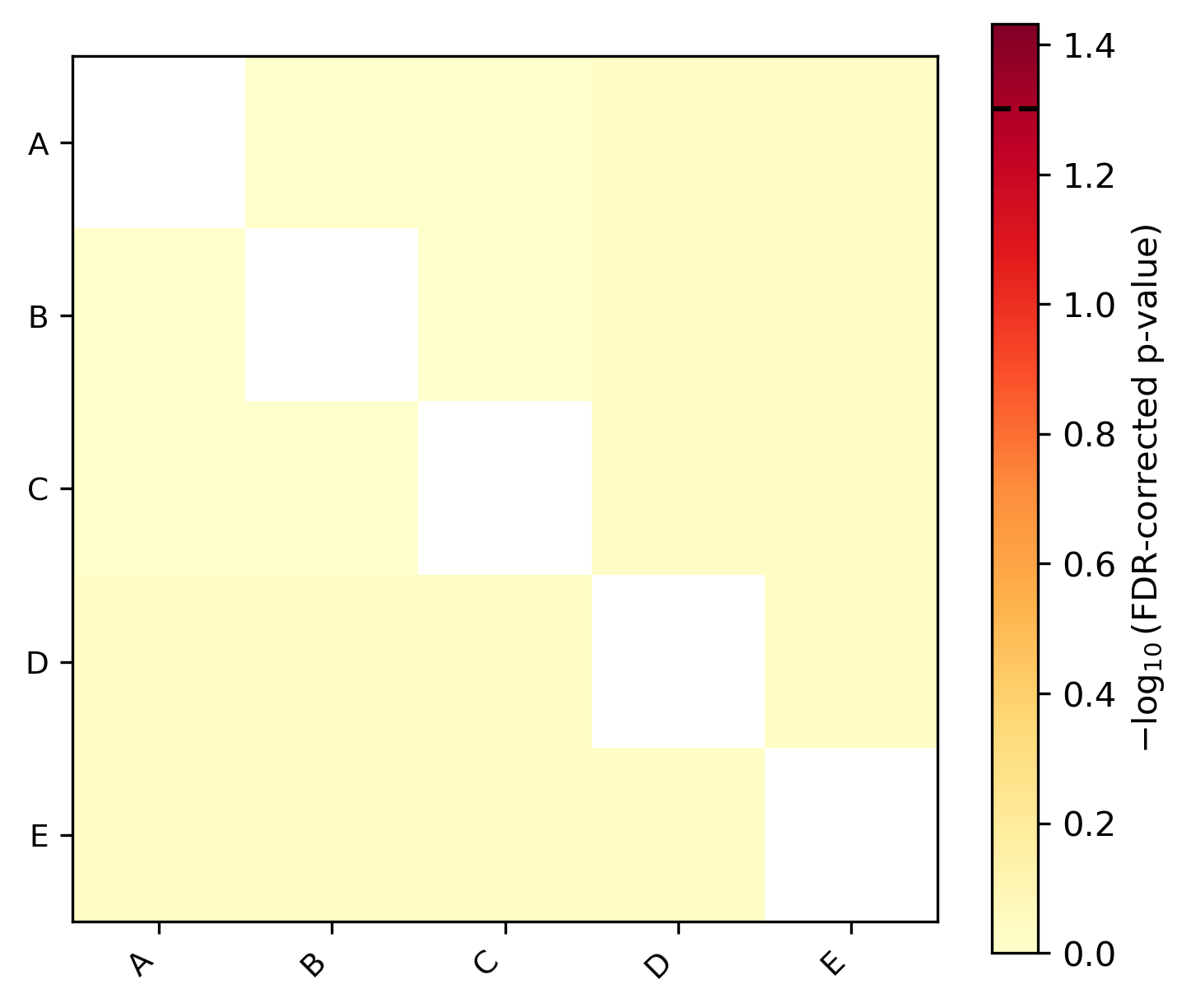
Unequal rates — taxa B and C have accumulated many more substitutions
than A and D. Significant pairs (dark red, marked with *) indicate
lineages evolving at detectably different rates:
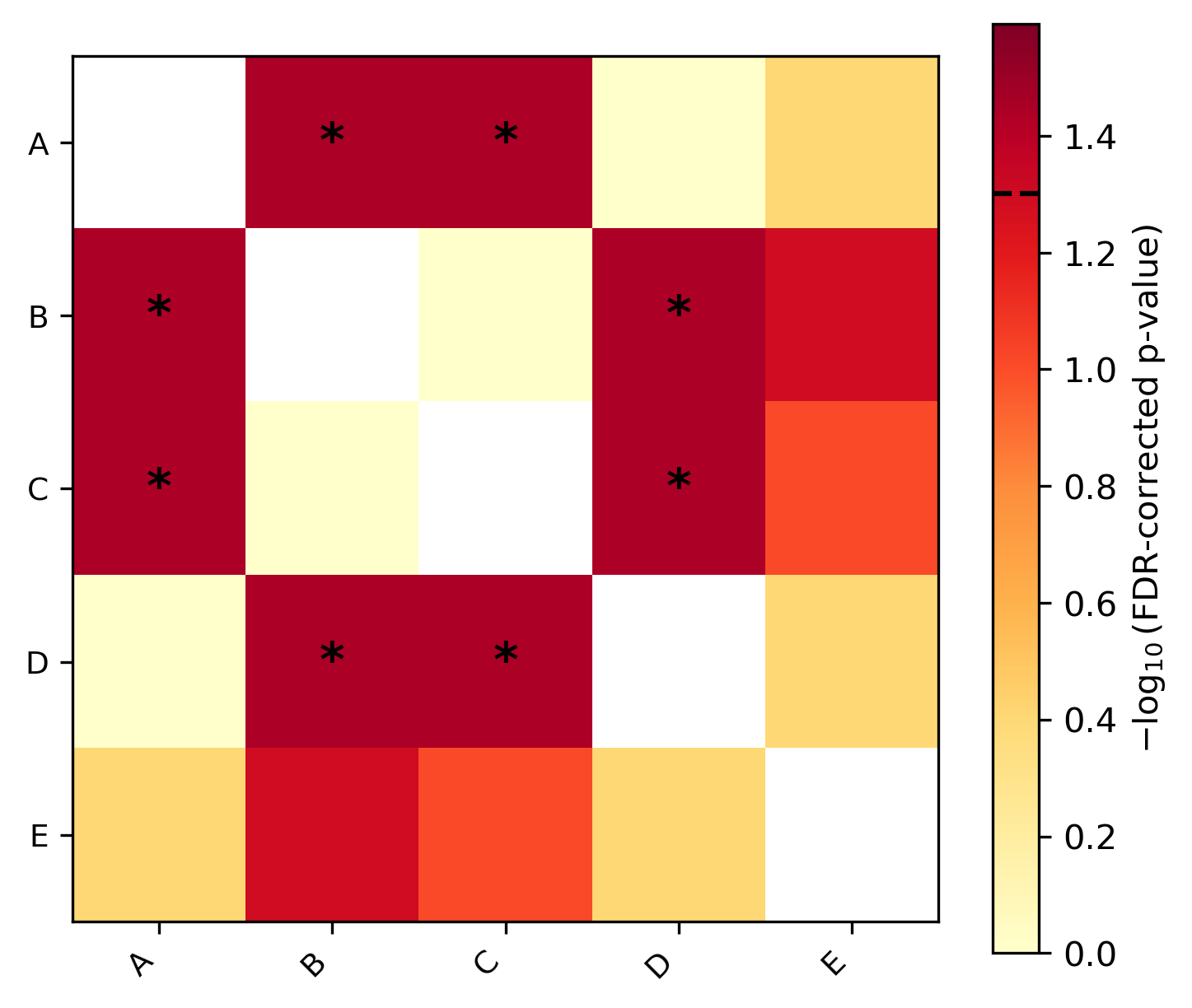
Validated against R's pegas::rr.test() — chi-squared and p-values
match to machine precision.
Saturation
Function names: saturation; sat
Command line interface: pk_saturation; pk_sat
Calculate saturation for a given tree and alignment.
Saturation is defined as sequences in multiple sequence alignments that have undergone numerous substitutions such that the distances between taxa are underestimated.
Data with no saturation will have a value of 1. The closer the value is to 1, the less saturated the data.
This function outputs two values (as of v1.19.9). The first value is the saturation value and the second column is the absolute value of saturation minus 1. Thus, lower values in the second column are indicative of values closer to one and, thus, less saturation.
Saturation is calculated following Philippe et al., PLoS Biology (2011), doi: 10.1371/journal.pbio.1000602.
phykit saturation -a <alignment> -t <tree> [-v/--verbose] [-e/--exclude_gaps] [--plot] [--plot-output <path>]
    [--fig-width <float>] [--fig-height <float>] [--dpi <int>] [--no-title] [--title <str>]
    [--legend-position <str>] [--ylabel-fontsize <float>] [--xlabel-fontsize <float>]
    [--title-fontsize <float>] [--axis-fontsize <float>] [--colors <str>] [--ladderize] [--cladogram] [--circular] [--color-file <file>] [--json]
Options:
-a/--alignment: an alignment file
-t/--tree: a tree file
-e/--exclude_gaps: if a site has a gap, ignore it
-v/--verbose: print out patristic distances and uncorrected
distances used to determine saturation
--plot: save a saturation scatter plot with fitted slope through origin
--plot-output: output path for saturation plot (default: saturation_plot.png)
--fig-width: figure width in inches (auto-scaled if omitted)
--fig-height: figure height in inches (auto-scaled if omitted)
--dpi: resolution in DPI (default: 300)
--no-title: hide the plot title
--title: custom title text
--legend-position: legend location (e.g., "upper right", "none" to hide)
--ylabel-fontsize: font size for y-axis labels; 0 to hide
--xlabel-fontsize: font size for x-axis labels; 0 to hide
--title-fontsize: font size for the title
--axis-fontsize: font size for axis labels
--colors: comma-separated colors (hex or named)
--ladderize: ladderize (sort) the tree before plotting
--cladogram: draw cladogram (equal branch lengths, tips aligned) instead of phylogram
--circular: draw circular (radial/fan) phylogram instead of rectangular
--color-file: color annotation file for tip labels, clade ranges, and branch colors (iTOL-inspired TSV format)
--json: optional argument to print results as JSON
Treeness over RCV
Function names: treeness_over_rcv; toverr; tor
Command line interface: pk_treeness_over_rcv; pk_toverr; pk_tor
Calculate treeness/RCV for a given alignment and tree.
Higher treeness/RCV values are thought to be desirable because they indicate a high signal-to-noise ratio and suggest the data are least susceptible to composition bias.
PhyKIT reports three tab delimited values: col1: treeness/RCV col2: treeness col3: RCV
Calculate treeness/RCV following Phillips and Penny, Molecular Phylogenetics and Evolution (2003), doi: 10.1016/S1055-7903(03)00057-5.
phykit treeness_over_rcv -a/--alignment <alignment> -t/--tree <tree> [--json]
Options:
-a/--alignment: an alignment file
-t/--tree: a tree file
--json: optional argument to print results as JSON