Tutorial 13: Testing for rate heterogeneity across phylogenetic regimes
Objectives
Complete the testing for rate heterogeneity across phylogenetic regimes workflow.
Interpret the reported values and generated artifacts in their scientific context.
Identify the canonical command references for each analysis step.
Prerequisites and working directory
Install the current PhyKIT release and create a dedicated working directory. Download the data linked in this tutorial into that directory before running the commands. All paths below are relative to this directory.
mkdir phykit-tutorial-13
cd phykit-tutorial-13
Workflow
A key question in comparative biology is whether the rate of trait evolution differs across lineages — for example, whether aquatic mammals evolve body size at a different rate than terrestrial mammals. Rate heterogeneity tests address this by fitting single-rate vs. multi-rate Brownian motion models and comparing them with a likelihood ratio test (O'Meara et al. 2006).
PhyKIT's rate_heterogeneity command (aliases: brownie, rh) implements
this test, analogous to R's phytools::brownie.lite().
Step 0: Prepare data
You need three input files:
A phylogenetic tree in Newick format
A tab-delimited trait file (
taxon<tab>value)A tab-delimited regime file (
taxon<tab>regime_label)
We will use the test data included with PhyKIT: an eight-taxon mammal phylogeny,
log-transformed body mass values, and regime assignments (aquatic vs. terrestrial).
Download test data:
Mammal phylogeny;
Continuous trait data;
Regime assignments
Step 1: Run the rate heterogeneity test
phykit rh -t tree_simple.tre -d tree_simple_traits.tsv -r tree_simple_regimes.tsv
Expected output:
Rate Heterogeneity Test (Multi-rate Brownian Motion)

Regimes: 2 (aquatic, terrestrial)
Number of tips: 8

Single-rate model (H0):
  Sigma-squared:      0.0384
  Ancestral state:    1.6447
  Log-likelihood:     -11.57
  AIC:                27.14

Multi-rate model (H1):
  Regime               Sigma-squared
  aquatic                     0.0088
  terrestrial                 0.0500
  Ancestral state:    1.8468
  Log-likelihood:     -11.20
  AIC:                28.41

Likelihood ratio test:
  LRT statistic:      0.7302
  Degrees of freedom: 1
  Chi-squared p-value: 0.3928

Effect size:
  R2_regime: -0.0341
Interpretation. The single-rate model estimates sigma-squared = 0.038 for all taxa. The multi-rate model estimates separate rates: aquatic mammals (sigma² = 0.009) evolve body mass more slowly than terrestrial mammals (sigma² = 0.050). However, the likelihood ratio test p-value of 0.39 is non-significant — we cannot reject the null hypothesis that rates are equal. The negative R²_regime (-0.03) confirms that the multi-rate model does not improve over the single-rate model. With only 2 aquatic taxa, power to detect rate differences is limited.
Step 2: Add a parametric bootstrap
For small sample sizes, the chi-squared approximation may be unreliable. Use the
-n flag to run a parametric bootstrap:
phykit rh -t tree_simple.tre -d tree_simple_traits.tsv -r tree_simple_regimes.tsv -n 100 --seed 42
The --seed flag ensures reproducibility.
Step 3: Generate a regime tree plot
Visualize which branches belong to which regime:
phykit rh -t tree_simple.tre -d tree_simple_traits.tsv -r tree_simple_regimes.tsv --plot regime_tree.png
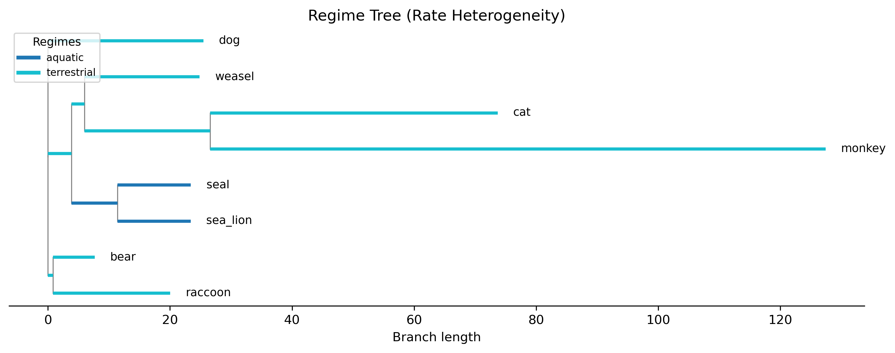
The plot shows the phylogeny with branches colored by regime assignment. Regime labels are inferred for internal branches using Fitch parsimony based on tip assignments. This visualization helps verify that the regime boundaries make biological sense.
Step 4: Export as JSON
phykit rh -t tree_simple.tre -d tree_simple_traits.tsv -r tree_simple_regimes.tsv --json
Summary
In this tutorial, we used the rate heterogeneity test to ask whether body mass evolves at different rates in aquatic vs. terrestrial mammals. The key steps were: (1) fitting single-rate and multi-rate BM models, (2) performing a likelihood ratio test, (3) optionally running a parametric bootstrap, and (4) visualizing regime assignments on the phylogeny.
For methodological details, see
O'Meara et al. (2006).
The R equivalent is phytools::brownie.lite()
(Revell 2012).
Expected artifacts
Each step identifies its expected terminal output or generated files. Confirm that those artifacts exist before continuing to the next step; filenames are relative to the tutorial working directory unless an absolute path is shown.
Troubleshooting
Run
phykit <command> --helpto compare an invocation with the live interface.Confirm that downloaded files are in the current working directory and retain the filenames shown in the tutorial.
For parsing errors, compare taxon names exactly across alignments, trees, and trait tables, including capitalization and underscores.
See Troubleshooting for installation, format, and error-reporting guidance.