Tutorial 7: Phylogenetic ordination for multivariate trait analysis
Objectives
Complete the phylogenetic ordination for multivariate trait analysis workflow.
Interpret the reported values and generated artifacts in their scientific context.
Identify the canonical command references for each analysis step.
Prerequisites and working directory
Install the current PhyKIT release and create a dedicated working directory. Download the data linked in this tutorial into that directory before running the commands. All paths below are relative to this directory.
mkdir phykit-tutorial-07
cd phykit-tutorial-07
Workflow
When analyzing multiple continuous traits across species, standard ordination methods ignore the phylogenetic non-independence among species: closely related species share evolutionary history and thus cannot be treated as independent data points. Phylogenetic ordination addresses this by incorporating the phylogenetic variance-covariance matrix, producing ordinations that properly account for shared ancestry.
PhyKIT's phylogenetic_ordination command (aliases: phylo_ordination, ordination,
ord, phylo_pca, phyl_pca, ppca, phylo_dimreduce, dimreduce, pdr)
supports three ordination methods:
PCA (default): phylogenetic PCA (Revell 2009) with Brownian motion or Pagel's lambda correction, and covariance or correlation modes
t-SNE: phylogenetically-corrected t-SNE for nonlinear dimensionality reduction
UMAP: phylogenetically-corrected UMAP for nonlinear dimensionality reduction
Hypothetical study question. Suppose we have measured body mass, brain size, and longevity for eight mammal species and want to identify the major axes of morphological variation while accounting for phylogenetic relationships. Which traits load most heavily on the primary axes? Do any species emerge as outliers after phylogenetic correction? Are there nonlinear patterns that PCA might miss?
Download test data:
Mammal phylogeny;
Multi-trait data
Step 0: Prepare data
Two input files are needed: a phylogenetic tree and a tab-delimited multi-trait file with a header row. The trait file looks like this:
taxon        body_mass       brain_size      longevity
raccoon      1.04    1.60    1.28
bear 2.39    2.66    1.36
sea_lion     2.30    2.74    1.46
seal 1.88    2.45    1.60
monkey       0.60    1.85    2.00
cat  0.56    1.30    1.18
weasel       -0.30   0.85    1.04
dog  1.18    1.87    1.20
Download both files above into the tutorial working directory.
Step 1: Run phylogenetic PCA with Brownian motion
The default method is PCA with Brownian motion for the phylogenetic covariance structure:
phykit phylogenetic_ordination \
    -t tree_simple.tre \
    -d tree_simple_multi_traits.tsv
Eigenvalues:
     PC1     PC2     PC3
eigenvalue   0.080180        0.002924        0.000308
proportion   0.961261        0.035052        0.003687

Loadings:
     PC1     PC2     PC3
body_mass    -0.734739       -0.422613       -0.530619
brain_size   -0.527400       -0.136064       0.838651
longevity    -0.426623       0.896038        -0.122915

Scores:
     PC1     PC2     PC3
bear -0.978191       -0.029290       -0.026787
cat  1.442009        0.176467        -0.093072
dog  0.651723        -0.091427       0.046142
monkey       0.640466        1.097251        0.208068
raccoon      0.867121        0.067199        -0.114611
sea_lion     -0.860400       -0.199268       0.115102
seal -0.522584       0.277539        0.059107
weasel       2.639715        -0.088806       0.080512
Interpretation. PC1 explains 96.1% of the total phylogenetically-corrected variance and loads most heavily on body mass (-0.73), followed by brain size (-0.53) and longevity (-0.43). This suggests that a single axis of overall body size captures most of the morphological variation. Weasel (score = 2.64) and cat (1.44) are the strongest outliers on PC1, reflecting their small body size, brain size, and short longevity relative to the larger-bodied species. PC2 (3.5% variance) is dominated by longevity (0.90), separating monkey (high longevity) from the other species.
Step 2: Use correlation mode
When traits are measured on different scales, correlation-mode PCA is often preferred because it standardizes each trait to unit variance before decomposition:
phykit ordination \
    -t tree_simple.tre \
    -d tree_simple_multi_traits.tsv \
    --mode corr
Eigenvalues:
     PC1     PC2     PC3
eigenvalue   2.849006        0.140247        0.010747
proportion   0.949669        0.046749        0.003582
Correlation-mode eigenvalues sum to the number of traits (3.0) rather than total variance. The loadings and scores change accordingly, but the overall pattern remains similar.
Step 3: Estimate Pagel's lambda jointly
Instead of assuming pure Brownian motion, the lambda correction jointly estimates Pagel's lambda across all traits, downweighting the phylogenetic covariance structure if the data warrant it:
phykit ordination \
    -t tree_simple.tre \
    -d tree_simple_multi_traits.tsv \
    --correction lambda \
    --json
The JSON output includes the estimated lambda value, eigenvalues, loadings, scores, and log-likelihood. A lambda near 1 indicates that Brownian motion adequately describes the covariance structure, while a lambda near 0 suggests traits evolved independently of phylogeny.
Step 4: Generate a PCA plot
To visualize the ordination, use the --plot flag:
phykit ordination \
    -t tree_simple.tre \
    -d tree_simple_multi_traits.tsv \
    --plot --plot-output ppca_plot.png
This generates a scatter plot of PC1 vs PC2 with taxon labels and variance-explained percentages on the axes.
Step 5: Nonlinear ordination with t-SNE and UMAP
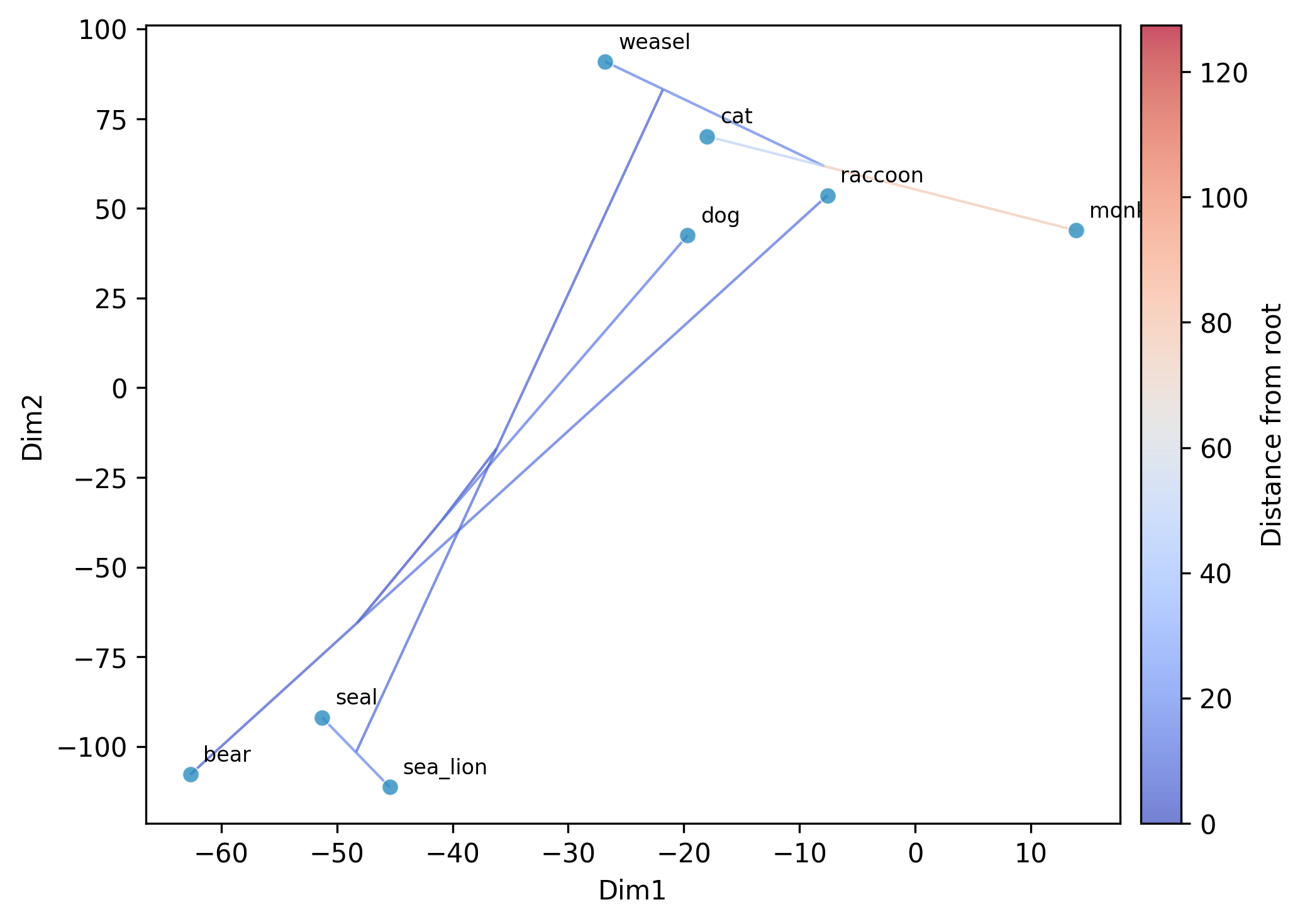
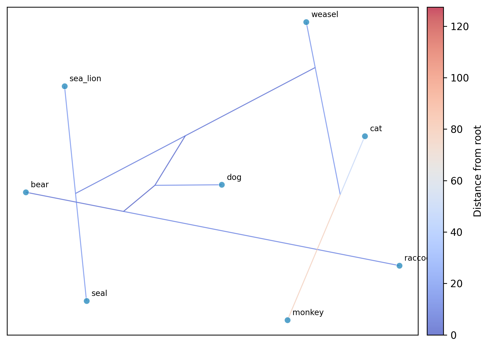
While PCA provides a linear ordination, nonlinear methods like t-SNE and UMAP can
reveal additional structure in high-dimensional trait spaces. The same GLS-centering
is applied before the nonlinear embedding. For t-SNE and UMAP, the phylogeny is
overlaid on the plot by default (edges colored by distance from root). Use
--no-plot-tree to disable this, or --tree-color-by to color edges by a trait
instead of distance from root. UMAP axes are unlabeled since the coordinates are
not directly interpretable.
Running t-SNE:
phykit ordination \
    -t tree_simple.tre \
    -d tree_simple_multi_traits.tsv \
    --method tsne --seed 42 --plot
Running UMAP:
phykit ordination \
    -t tree_simple.tre \
    -d tree_simple_multi_traits.tsv \
    --method umap --seed 42 --plot
Using Pagel's lambda correction with t-SNE:
phykit ordination \
    -t tree_simple.tre \
    -d tree_simple_multi_traits.tsv \
    --method tsne --correction lambda --seed 42 --json
Coloring phylogeny edges by a trait (e.g., body_mass) instead of distance from root:
phykit ordination \
    -t tree_simple.tre \
    -d tree_simple_multi_traits.tsv \
    --method tsne --plot --tree-color-by body_mass --seed 42
Disabling the phylogeny overlay:
phykit ordination \
    -t tree_simple.tre \
    -d tree_simple_multi_traits.tsv \
    --method umap --plot --no-plot-tree --seed 42
Summary
In this tutorial, we used phylogenetic ordination to identify the major axes of morphological variation among mammal species while accounting for shared evolutionary history. The key steps were: (1) running PCA under Brownian motion, (2) comparing covariance and correlation modes, (3) jointly estimating Pagel's lambda, (4) visualizing the ordination, and (5) exploring nonlinear structure with t-SNE and UMAP.
For PCA methodological details, see
Revell (2009).
The R equivalent is phytools::phyl.pca()
(Revell 2012).
Expected artifacts
Each step identifies its expected terminal output or generated files. Confirm that those artifacts exist before continuing to the next step; filenames are relative to the tutorial working directory unless an absolute path is shown.
Troubleshooting
Run
phykit <command> --helpto compare an invocation with the live interface.Confirm that downloaded files are in the current working directory and retain the filenames shown in the tutorial.
For parsing errors, compare taxon names exactly across alignments, trees, and trait tables, including capitalization and underscores.
See Troubleshooting for installation, format, and error-reporting guidance.