Tutorial 19: End-to-end comparative methods workflow
Objectives
Complete the end-to-end comparative methods workflow workflow.
Interpret the reported values and generated artifacts in their scientific context.
Identify the canonical command references for each analysis step.
Prerequisites and working directory
Install the current PhyKIT release and create a dedicated working directory. Download the data linked in this tutorial into that directory before running the commands. All paths below are relative to this directory.
mkdir phykit-tutorial-19
cd phykit-tutorial-19
Workflow
Phylogenetic comparative methods are most powerful when used together. This tutorial demonstrates a complete workflow: testing for phylogenetic signal, comparing evolutionary models, fitting a regression, and visualizing results — all using PhyKIT.
Scenario
Imagine you have assembled a phylogeny of eight mammal species and measured their body mass and brain size. You want to answer a classic question in comparative biology: does body mass predict brain size after controlling for shared evolutionary history? Before testing this relationship, you need to verify that your traits have phylogenetic signal (justifying the use of phylogenetic methods) and determine which evolutionary model best describes how body mass has evolved. Finally, you want publication-ready figures that show trait evolution on the phylogeny and visualize the brain-body relationship in phylogenetic morphospace.
Overview
We will use an eight-taxon mammal tree and body-mass trait data to:
Test whether body mass has phylogenetic signal (
phylogenetic_signal)Compare models of trait evolution (
fit_continuous)Ask whether body mass predicts brain size (
pgls)Visualize results (
cont_map,phenogram,phylomorphospace)
Data files used in this tutorial:
Download test data:
Mammal phylogeny;
Continuous trait data (body mass);
Multi-trait data (body mass, brain size, longevity)
tree_simple.tre— an eight-taxon mammal phylogeny in Newick formattree_simple_traits.tsv— body mass (log-transformed kg), tab-delimited with taxon and value columns (no header, lines starting with#are comments)tree_simple_multi_traits.tsv— body mass, brain size, and longevity, tab-delimited with a header row
Step 1: Test for phylogenetic signal
Before running any comparative analysis, check whether the trait shows phylogenetic signal — i.e., whether closely related species have more similar trait values than expected by chance. For our mammal dataset, we expect body mass to show strong phylogenetic signal because closely related mammals tend to have similar body sizes.
phykit phylogenetic_signal -t tree_simple.tre -d tree_simple_traits.tsv
Expected output:
0.5842 0.474 0.9499
col1: Blomberg's K
col2: p-value (from permutation test)
col3: R²_phylo, the relative reduction in fitted variance under Brownian
motion compared with a white-noise model
Here, K = 0.58 and the permutation p-value of 0.474 is non-significant
with these 8 taxa. R²_phylo = 0.95 indicates that the Brownian-motion
model has substantially lower fitted variance than the white-noise model.
It is not an estimate of Pagel's lambda; calculate lambda explicitly with
-m lambda as shown in Tutorial 6.
What if signal is weak? A K near 0 with a non-significant permutation test provides little evidence for phylogenetic signal in this analysis. Model choice should consider the signal estimate, uncertainty, sample size, and assumptions of the downstream analysis.
For JSON output including the effect size (R² phylo):
phykit phylogenetic_signal -t tree_simple.tre -d tree_simple_traits.tsv --json
{"K": 0.5842, "p_value": 0.474, "permutations": 1000, "r_squared_phylo": 0.9499}
The r_squared_phylo value compares the fitted Brownian-motion variance
with the white-noise variance. It should not be interpreted as the literal
percentage of trait variance caused by phylogenetic relatedness.
Step 2: Compare evolutionary models
Next, determine which model of continuous trait evolution best explains the observed body-mass data. This helps interpret how body mass has evolved across these mammals — did it drift randomly (Brownian motion), was it pulled toward an optimal size (OU), or did most change happen early in the clade's history (Early Burst)?
phykit fit_continuous -t tree_simple.tre -d tree_simple_traits.tsv
Expected output:
Model Comparison (fitContinuous)

Number of tips: 8

Model       Param     Value      Sigma2    z0        LL         AIC      dAIC     AICw     BIC      dBIC     R2
White       -         -          0.7667    1.2062    -10.289    24.58    0.00     0.304    24.74    0.00     0.000
EB          a         -0.0785    0.0854    1.4827    -9.595     25.19    0.61     0.224    25.43    0.69     0.889
Kappa       kappa     0.0100     0.3428    1.3230    -9.722     25.44    0.87     0.197    25.68    0.94     0.553
OU          alpha     0.7848     1.2035    1.2063    -10.289    26.58    2.00     0.112    26.82    2.08     -0.570
BM          -         -          0.0384    1.6447    -11.570    27.14    2.56     0.084    27.30    2.56     0.950
Delta       delta     0.5188     0.1968    1.4939    -11.128    28.26    3.68     0.048    28.49    3.76     0.743
Lambda      lambda    1.0000     0.0384    1.6447    -11.570    29.14    4.56     0.031    29.38    4.64     0.950

Best model (AIC): White
Best model (BIC): White
Models are ranked by AIC (lower is better). The dAIC column shows the
difference from the best model, and AICw gives the Akaike weight
(probability of being the best model). The R2 column shows each model's
effect size relative to the White (no phylogenetic structure) model. In
this small dataset, the White model wins by AIC, but BM has R² = 0.95,
indicating that BM explains most trait variance — with more taxa, BM
would likely be preferred.
To compare only a subset of models:
phykit fc -t tree_simple.tre -d tree_simple_traits.tsv --models BM,OU,Lambda
Step 3: Test a trait-trait relationship with PGLS
Now we arrive at the central question: does body mass predict brain size? A naive correlation would be misleading because closely related species share both large bodies and large brains simply due to common descent. PGLS (phylogenetic generalized least squares) controls for this non-independence.
phykit pgls -t tree_simple.tre -d tree_simple_multi_traits.tsv -y brain_size -x body_mass
Expected output:
Phylogenetic Generalized Least Squares (PGLS)

Formula: brain_size ~ body_mass

Coefficients:
                        Estimate   Std.Error     t-value     p-value
(Intercept)               0.9972      0.0871     11.4467    0.000027    ***
body_mass                 0.7086      0.0451     15.7140    0.000004    ***
---
Signif. codes:  0 '***' 0.001 '**' 0.01 '*' 0.05 '.' 0.1

Residual standard error: 0.0250 on 6 degrees of freedom
Multiple R-squared: 0.9763    Adjusted R-squared: 0.9723
R-squared (total):   0.9988   (phylo + predictor)
R-squared (phylo):   0.0225   (phylogeny contribution)
F-statistic: 246.93 on 1 and 6 DF    p-value: 0.000004
Log-likelihood: 6.0558    AIC: -6.1117
The slope of 0.71 means that for every 1-unit increase in log body mass,
log brain size increases by 0.71 — consistent with allometric scaling.
The p-value (0.000004) is highly significant. The R² decomposition reveals
that body mass explains 97.6% of brain-size variance (r_squared),
while phylogenetic relatedness alone explains only 2.3%
(r_squared_phylo). The total R² of 99.9% (r_squared_total)
captures both sources combined.
For JSON output:
phykit pgls -t tree_simple.tre -d tree_simple_multi_traits.tsv -y brain_size -x body_mass --json
Step 4: Visualize trait evolution
Finally, generate publication-ready figures. Visualization often reveals patterns that summary statistics miss — for example, a contMap might show that large body mass evolved independently in two distant clades, or a phylomorphospace might reveal an outlier species that departs from the brain-body allometry.
contMap — paint continuous body-mass values onto the phylogeny, showing where evolutionary increases and decreases occurred:
phykit cont_map -t tree_simple.tre -d tree_simple_traits.tsv -o body_mass_contmap.png
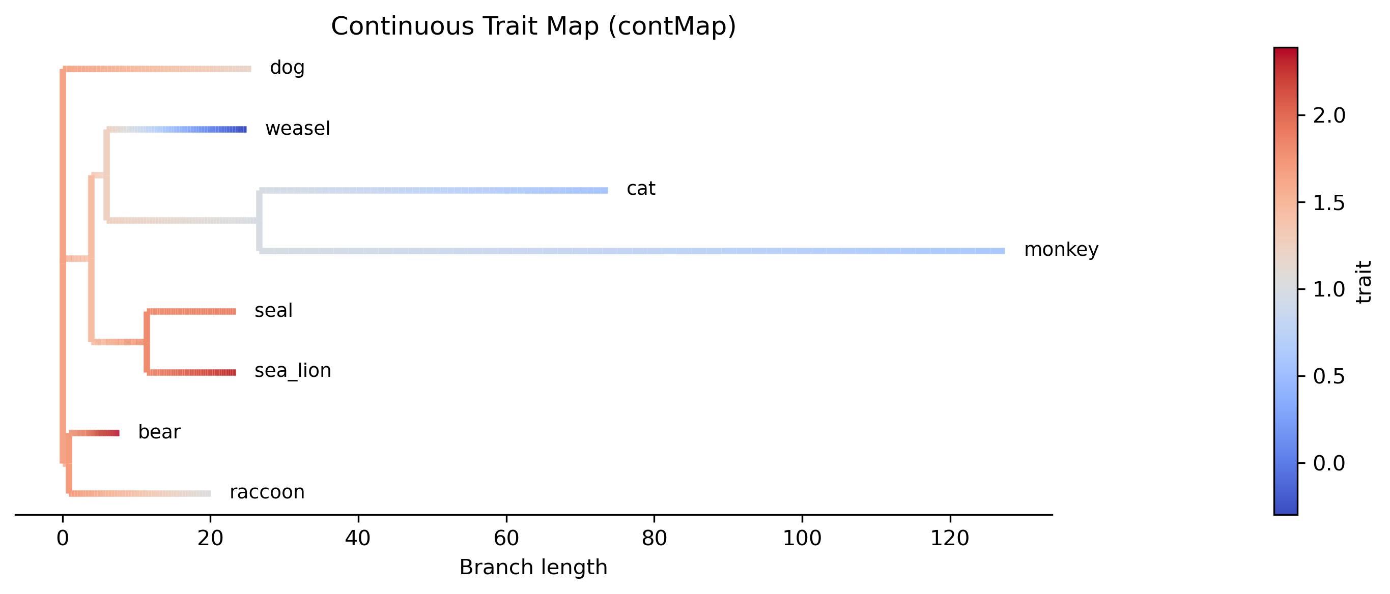
The contMap shows body mass reconstructed along each branch using Brownian motion. Warm colors indicate high body mass (bear, sea lion) while cool colors indicate low body mass (weasel). The color gradient along branches shows where evolutionary changes occurred.
phenogram — plot body-mass values against distance from the root, revealing whether trait change was gradual or punctuated:
phykit phenogram -t tree_simple.tre -d tree_simple_traits.tsv -o body_mass_phenogram.png
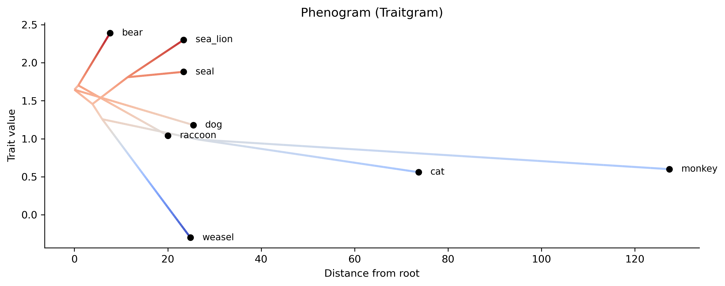
The phenogram (traitgram) plots trait values on the y-axis against evolutionary time on the x-axis. Lineages trace from their common ancestor to tips, revealing the tempo and mode of body-mass evolution. Closely related species (e.g., bear and raccoon) converge toward their common ancestor's value.
phylomorphospace — visualize body mass and brain size simultaneously in phylogenetic space, with branches connecting ancestors to descendants:
phykit phylomorphospace -t tree_simple.tre -d tree_simple_multi_traits.tsv \
    --trait-x body_mass --trait-y brain_size --plot-output morphospace.png
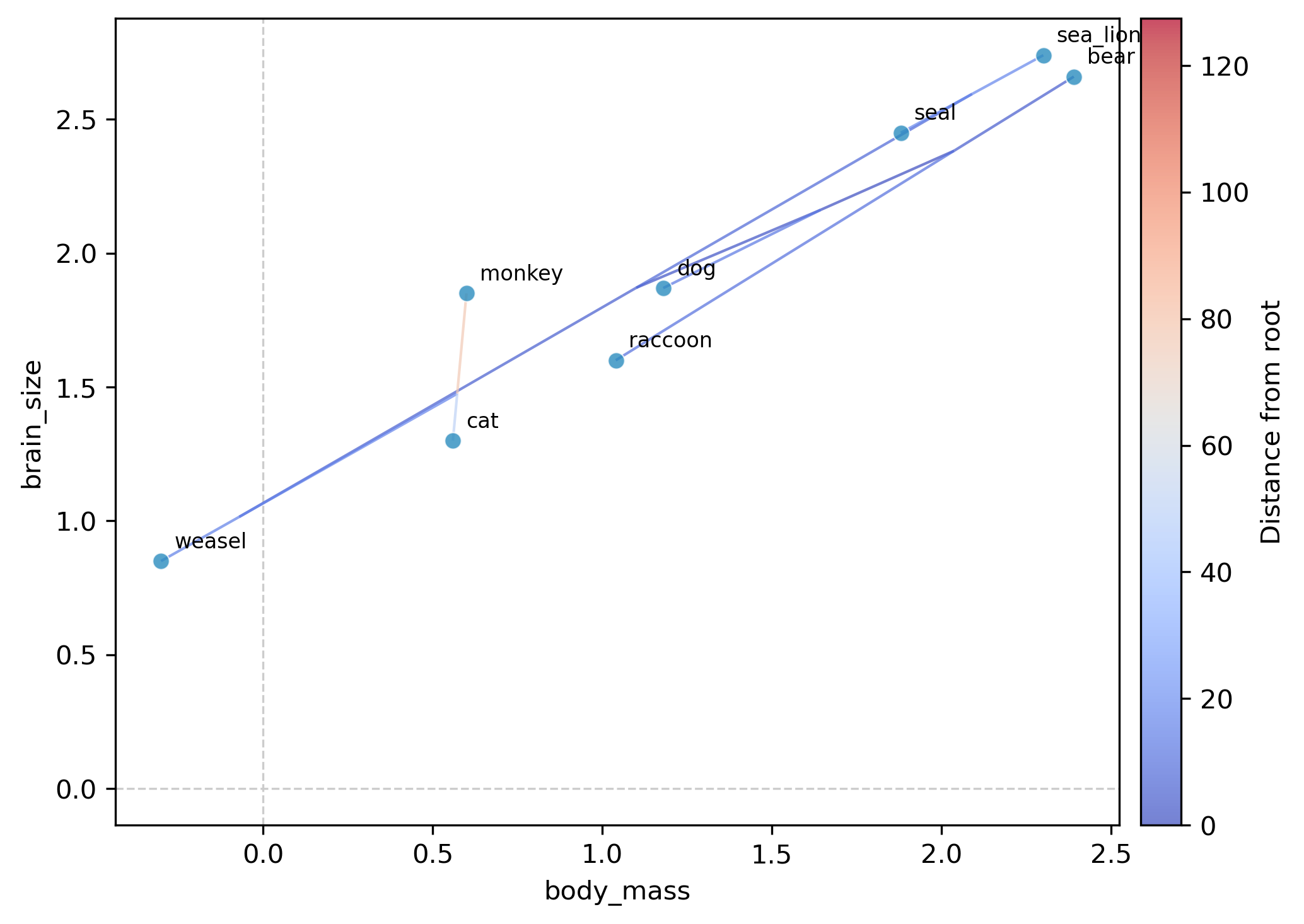
The phylomorphospace plots each species as a point in body-mass × brain-size space, with branches connecting species through their reconstructed ancestors. The tight clustering along the diagonal confirms the strong allometric relationship detected by PGLS. The monkey stands apart from the carnivore cluster, reflecting its distinct clade membership.
Putting it all together
Returning to our mammal example, a typical analysis would proceed as:
Phylogenetic signal? Body mass shows strong signal (K > 1, lambda ≈ 1), confirming that phylogenetic methods are necessary.
Which evolutionary model? If BM fits best, body mass drifted randomly; if OU wins, mammals are evolving toward a preferred body size. This shapes how we interpret downstream results.
Trait-trait association? PGLS confirms that body mass predicts brain size even after accounting for phylogeny. The R² decomposition tells us how much of brain-size variation is explained by body mass vs. by phylogenetic relatedness alone.
Visualization — the contMap shows where on the tree body mass increased, the phenogram reveals the tempo of change, and the phylomorphospace shows whether species cluster by clade or by ecological niche in brain-body space.
This workflow generalizes to any trait and phylogeny: substitute your own tree, trait data, and biological question.
Expected artifacts
Each step identifies its expected terminal output or generated files. Confirm that those artifacts exist before continuing to the next step; filenames are relative to the tutorial working directory unless an absolute path is shown.
Troubleshooting
Run
phykit <command> --helpto compare an invocation with the live interface.Confirm that downloaded files are in the current working directory and retain the filenames shown in the tutorial.
For parsing errors, compare taxon names exactly across alignments, trees, and trait tables, including capitalization and underscores.
See Troubleshooting for installation, format, and error-reporting guidance.