Tutorial 11: Reconstructing ancestral trait values and mapping them onto a phylogeny
Objectives
Complete the reconstructing ancestral trait values and mapping them onto a phylogeny workflow.
Interpret the reported values and generated artifacts in their scientific context.
Identify the canonical command references for each analysis step.
Prerequisites and working directory
Install the current PhyKIT release and create a dedicated working directory. Download the data linked in this tutorial into that directory before running the commands. All paths below are relative to this directory.
mkdir phykit-tutorial-11
cd phykit-tutorial-11
Workflow
A common question in comparative biology is: what were the trait values of ancestral species? Ancestral state reconstruction (ASR) uses the trait values observed at the tips of a phylogeny together with a model of trait evolution to estimate what trait values were at each internal node.
PhyKIT's ancestral_state_reconstruction command (aliases: asr,
anc_recon) supports both continuous and discrete traits:
Continuous (
--type continuous, default): Brownian Motion model with two ML methods —fast(Felsenstein's pruning, analogous tophytools::fastAnc()) andml(full VCV-based ML with exact CIs, analogous toape::ace(type="ML")).Discrete (
--type discrete): Mk model with marginal posterior probabilities at each internal node, analogous toape::ace(type="discrete"). Three models are available:ER(equal rates),SYM(symmetric), andARD(all rates different).
Hypothetical study question. Given body mass data for 8 mammal species,
what were the estimated body masses of their ancestors? And given dietary
categories (carnivore, herbivore, omnivore), what were the most likely diets
of ancestral species?
Download test data:
Mammal phylogeny;
Trait data;
Multi-trait data;
Discrete trait data
Step 0: Prepare data
Two input files are needed: a phylogenetic tree and a trait data file.
The trait data can be either a two-column file (taxon<tab>value) or
a multi-trait file with a header row (use -c to select a column).
Step 1: Run fast ancestral reconstruction with confidence intervals
Estimate ancestral body masses using the fast (two-pass Felsenstein) method with 95% confidence intervals:
phykit ancestral_state_reconstruction \
    -t tree_simple.tre \
    -d tree_simple_traits.tsv \
    --ci
Ancestral State Reconstruction

Method: fast (Felsenstein's contrasts)
Trait: trait
Number of tips: 8

Log-likelihood: -11.6038
Sigma-squared (BM rate): 0.043893

Ancestral estimates:
  Node         Descendants    Estimate                  95% CI
  N1 (root)              8      1.6447        [0.8937, 2.3957]
  N2                     2      1.7012        [0.9697, 2.4328]
  N3                     5      1.4565        [0.6387, 2.2742]
  N4                     2      1.8091        [0.9757, 2.6425]
  N5                     3      1.2566        [0.3555, 2.1577]
  N6                     2      0.9895       [-0.5654, 2.5443]
Interpretation. The root ancestor (N1) is estimated to have had a log body mass of 1.64 (95% CI: 0.89 -- 2.40). Node N6 (the ancestor of cat and monkey) has the widest confidence interval [-0.57, 2.54], reflecting the long branch lengths separating these taxa. Node N4 (sea_lion + seal ancestor) has the highest estimate (1.81), consistent with these being the largest-bodied members of that clade.
Step 2: Use the VCV-based ML method
For exact conditional confidence intervals computed from the full
phylogenetic variance-covariance matrix, use the ml method:
phykit asr \
    -t tree_simple.tre \
    -d tree_simple_traits.tsv \
    -m ml --ci
Both methods produce identical point estimates. The ml method computes CIs
from the conditional distribution of internal node values given the observed
tips, while fast uses the pruning-based variance. For bifurcating trees
the CIs are identical; for polytomies they may differ slightly.
Step 3: Generate a contMap plot
The --plot option produces a contMap visualization analogous to R's
phytools::contMap(). Branches are colored by a continuous gradient
representing the interpolated trait value from the parent's estimate to the
child's estimate:
phykit asr \
    -t tree_simple.tre \
    -d tree_simple_traits.tsv \
    --plot contmap.png
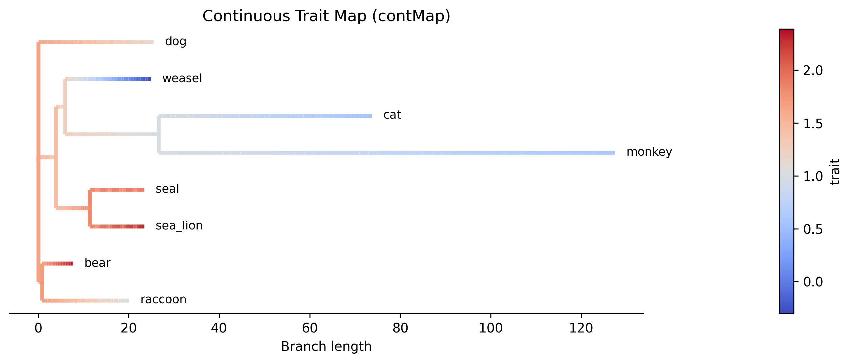
Interpretation. The contMap shows how log body mass varies across the phylogeny. Warm colors (red) indicate higher body mass values, while cool colors (blue) indicate lower values. The gradient along each branch reflects the linear interpolation between the parent and child ancestral estimates. The bear + raccoon clade (top) shows uniformly warm colors consistent with high body mass, while the weasel lineage transitions toward cooler colors reflecting its much lower body mass (-0.30). The cat + monkey clade shows moderate values transitioning from the ancestral estimate.
The contMap can be combined with --ci and -m ml to use a specific
method for the underlying reconstruction, or with -c to select a trait
from a multi-trait file:
phykit asr \
    -t tree_simple.tre \
    -d tree_simple_multi_traits.tsv \
    -c brain_size --plot brain_contmap.png --ci
Step 4: Use a multi-trait file
When your data file contains multiple traits with a header row, use
-c to select a specific column:
phykit asr \
    -t tree_simple.tre \
    -d tree_simple_multi_traits.tsv \
    -c body_mass --ci
Step 5: Export results as JSON
For downstream scripting, results can be exported as JSON:
phykit asr \
    -t tree_simple.tre \
    -d tree_simple_traits.tsv \
    --json
The JSON output includes the method used, trait name, number of tips, log-likelihood, sigma-squared (BM rate), ancestral estimates with optional CIs, and observed tip values.
Step 6: Reconstruct discrete traits
For discrete (categorical) traits, use --type discrete. This fits an
Mk model and computes marginal posterior probabilities at each internal
node using upward-downward belief propagation:
phykit asr \
    -t tree_simple.tre \
    -d tree_simple_discrete_traits.tsv \
    -c diet --type discrete
Ancestral State Reconstruction (Discrete)

Model: Mk (ER)
Trait: diet
Number of tips: 8
Number of states: 3
States: carnivore, herbivore, omnivore

Log-likelihood: -8.7874

Rate matrix (Q):
                 carnivore   herbivore    omnivore
     carnivore   -0.113825    0.056912    0.056912
     herbivore    0.056912   -0.113825    0.056912
      omnivore    0.056912    0.056912   -0.113825

Ancestral state posteriors:
  Node          Desc        MAP  carnivore  herbivore   omnivore
  N1 (root)        8  carnivore     0.5338     0.2294     0.2368
  N2               2  carnivore     0.5662     0.2140     0.2199
  N3               5  carnivore     0.4381     0.2806     0.2813
  N4               2  carnivore     0.3988     0.3516     0.2496
  N5               3  carnivore     0.3994     0.2906     0.3100
  N6               2  carnivore     0.3352     0.3320     0.3329
Interpretation. The output shows the fitted rate matrix (Q) and marginal posterior probabilities for each state at every internal node. The MAP (maximum a posteriori) column gives the most likely state. Under the equal-rates model, the root (N1) is most likely carnivore (posterior 0.53). Node N6 (cat + monkey ancestor) shows nearly uniform posteriors across all three states, reflecting uncertainty.
Step 7: Choose a discrete model
The --model flag selects the Mk model variant:
ER(default): all transition rates equalSYM: forward and reverse rates between each pair of states are equalARD: all rates differ (most parameter-rich)
phykit asr \
    -t tree_simple.tre \
    -d tree_simple_discrete_traits.tsv \
    -c diet --type discrete --model ARD
Compare log-likelihoods across models to assess fit. With only 8 tips and
3 states, the simpler ER model is often preferred to avoid overfitting.
Step 8: Plot discrete ancestral states
The --plot option for discrete traits produces a phylogeny with pie
charts at internal nodes showing the posterior probabilities for each state:
phykit asr \
    -t tree_simple.tre \
    -d tree_simple_discrete_traits.tsv \
    -c diet --type discrete --plot discrete_asr.png
Tip labels are colored by their observed state, and a legend maps colors to
state names. This is analogous to the pie-chart plots commonly used in R
with ape::plot.phylo() and ape::nodelabels(pie=...).
Summary
In this tutorial, we used ancestral state reconstruction for both continuous and discrete traits. For continuous traits, the key steps were: (1) running the fast method with confidence intervals, (2) using the full ML method for exact conditional CIs, (3) generating contMap plots, (4) using multi-trait files, and (5) exporting to JSON. For discrete traits, we (6) reconstructed ancestral dietary categories with posterior probabilities, (7) compared different Mk model variants, and (8) generated pie-chart phylogeny plots.
For continuous traits, the fast method is recommended for large trees
due to its O(n) time complexity, while ml provides exact conditional
confidence intervals at O(n^3) cost. Both produce identical point estimates
matching R's phytools::fastAnc() to machine precision.
For discrete traits, the ER model is a good default; use SYM or
ARD when you have reason to expect asymmetric transition rates and
sufficient tip data to estimate extra parameters.
The R equivalents are phytools::fastAnc() for continuous fast,
ape::ace(type="ML") for continuous ML, phytools::contMap() for
contMap plots, and ape::ace(type="discrete") for discrete ASR.
Expected artifacts
Each step identifies its expected terminal output or generated files. Confirm that those artifacts exist before continuing to the next step; filenames are relative to the tutorial working directory unless an absolute path is shown.
Troubleshooting
Run
phykit <command> --helpto compare an invocation with the live interface.Confirm that downloaded files are in the current working directory and retain the filenames shown in the tutorial.
For parsing errors, compare taxon names exactly across alignments, trees, and trait tables, including capitalization and underscores.
See Troubleshooting for installation, format, and error-reporting guidance.